Attractive Stepping Stones Landscapes: Preference for Stone Height Variation Appears to Be Age Independent

Figures & data

Table 1. The anthropometrics (means and standard deviations) of the 26 young and 25 older adults participating in Experiment 1.

Group	Gender	Age (years)	Leg length (cm)
Young adults	19F / 7M	22.15 ± 2.12	90.31 ± 5.82
Older adults	18F / 7M	70.75 ± 5.40	87.60 ± 5.99

Figure 1. Arrangement of the jumping stone configurations in Experiment 1. All numbers represent gap widths in cm. The gap widths between the middle of the landscape and each of the configurations was 222.5 cm (as shown for the ‘standard’ configuration).

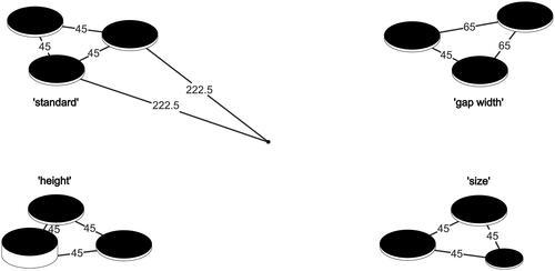
Figure 2. The medians (dots) and interquartile ranges (25-75^th percentile) of the judgment scores of the configurations in Experiment 1. The higher the scores, the more fun, esthetically appealing, challenging and risky a configuration was judged. * indicates a significant difference at p < .05.

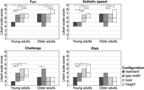
Table 2. The means and standard deviations of the maximum jumping distance and TUG scores of the 26 young and 25 older adults participating in Experiment 1.

Group	Max. stepping distance (cm)	TUG test (s)
Young adults	116.85 ± 12.91	7.26 ± 0.80
Older adults	98.32 ± 11.22	8.28 ± 1.37

Table 3. Kendall’s tau correlation matrix of the subjective judgments for each configuration and age group in Experiment 1.

		Young adults			Older adults
Config.	Subj. Judgm.	1.	2.	3.	1.	2.	3.
‘standard’	1. Fun
	2. Esthet. appeal	.482**			.679**
	3. Challenge	−.112	−.145		.005	.064
	4. Risk	−.017	−.077	.018	.114	.028	.583**
‘gap width’	1. Fun
	2. Esthet. appeal	.322^a			.603**
	3. Challenge	.088	.267		−.227	−.238
	4. Risk	.307	.185	.355*	−.090	.055	.528**
‘size’	1. Fun
	2. Esthet. appeal	.214			.480**
	3. Challenge	.083	−.200		−.168	−.121
	4. Risk	−.152	.012	.415**	.023	.112	.673**
‘height’	1. Fun
	2. Esthet. appeal	.339*			.450**
	3. Challenge	.248	.202		−.078	−.199
	4. Risk	.181	.385*	.433**	.055	.156	.502**

* and ** indicate significant correlations at respectively at p < .05 and p < .01. ^a indicates a marginally significant correlation at p = .052.

Figure 3. For both young and older adults clockwise from the upper left: the ‘standard’ configuration, ‘size’ configuration, ‘gap width’ configuration, and ‘height’ configuration (hatched circle represents the higher stone). Next to each gap we present the average number of crossings as a percentage of the total number of gap crossings (number of times the gap was crossed/ total number of gap crossings * 100)². The thicker the line of the gap, the more frequently the gap was crossed. In addition, the medians and interquartile ranges of the number of play bouts are presented for each configuration.

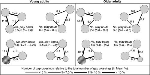
Figure 4. Violin plot with the medians (solid line) and interquartile ranges (dotted lines) of the playtime spent by young and older adults in each configuration of Experiment 1. * indicates a significant difference at p < .05.

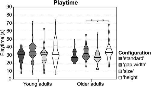
Figure 5. Violin plot with the medians (solid line) and interquartile ranges (dotted lines) of the total number of gap crossings of young and older adults in each configuration, and the number of gap crossings per minute in each configuration for both groups in Experiment 1. * indicates a significant difference at p < .05.

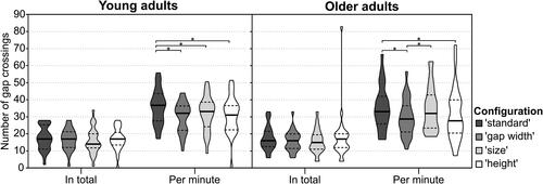
Table 4. The anthropometrics (means and standard deviations) of the 25 young and 28 older adults participating in Experiment 2.

Group	Gender	Age (years)	Leg length (cm)
Young adults	14F / 11M	21.52 ± 2.01	90.98 ± 4.82
Older adults	16F / 12M	70.08 ± 5.62	88.38 ± 5.21

Figure 6. Arrangement of the jumping stone configurations in Experiment 2. All numbers represent gap widths in cm. The gap width between the middle and each of the configurations was 222.5 cm (as shown for the H configuration).

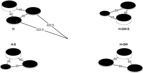
Figure 7. The medians (dots) and interquartile ranges (25-75^th percentile) of the judgment scores of the configurations in Experiment 2. The higher the scores, the more fun, esthetic appealing, challenging and risky a configuration was judged. * indicates a significant difference at p < .05.

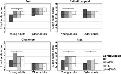
Table 5. The means and standard deviations of the maximum jumping distance and TUG scores of the 25 young and 28 older adults participating in Experiment 2.

Group	Max. stepping distance (cm)	TUG test (s)
Young adults	117.38 ± 12.17	7.14 ± 0.60
Older adults	94.09 ± 12.86	8.55 ± 1.41

Table 6. Kendall’s tau correlation matrix of the subjective judgments for each configuration and age group in Experiment 2.

		Young adults			Older adults
Config.	Subj. Judgm.	1.	2.	3.	1.	2.	3.
H-GW-S	1. Fun
	2. Esthet. appeal	.375*			.536**
	3. Challenge	−.049	−.267		−.038	−.153
	4. Risk	.107	−.008	.520**	−.041	−.220	.677**
H-GW	1. Fun
	2. Esthet. appeal	.092^a			.633**
	3. Challenge	.071	−.056		−.068	.003
	4. Risk	−.068	−.040	.549**	−.139	−.096	.645**
H-S	1. Fun	.403*			.389*
	2. Esthet. appeal	−.062	−.020		−.078	.015
	3. Challenge	.025	.049	.602**	.062	−.160	.615**
	4. Risk
H	1. Fun
	2. Esthet. appeal	.660**			.466**
	3. Challenge	.106	.125		−.061	−.164
	4. Risk	−.044	.024	.653**	.072	−.217	.609**

* and ** indicate significant correlations at respectively at p < .05 and p < .01. ^a Indicates a marginally significant correlation at p = .058.

Figure 8. For both young and older adults clockwise from the upper left: the H configuration, H-GW-S configuration, H-GW configuration, and H-S configuration (hatched circle represents the higher stone). Next to each gap we present the average number of crossings as a percentage of the total number of gap crossings (number of times the gap was crossed/ total number of gap crossings * 100)³. The thicker the line of the gap, the more frequently the gap was crossed. In addition, the medians and interquartile ranges of the number of play bouts are presented for each configuration.

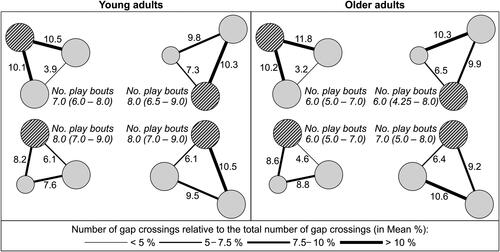
Figure 9. Violin plot with the medians (solid line) and interquartile ranges (dotted lines) of the total number of gap crossings of young and older adults in each configuration, and the number of gap crossings per minute in each configuration for both groups in Experiment 2. * indicates a significant difference at p < .05.

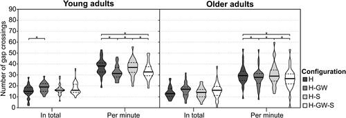
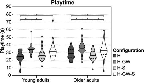
Figure 10. Violin plot with the medians (solid line) and interquartile ranges (dotted lines) of the playtime spent by young and older adults in each configuration of Experiment 2. * indicates a significant difference at p < .05.