Heat transfer and pressure drop correlations for laminar flow in an in-line and staggered array of circular cylinders

Figures & data

Figure 1. Concept of a flat tube heat exchanger with plate-fin wire structure.

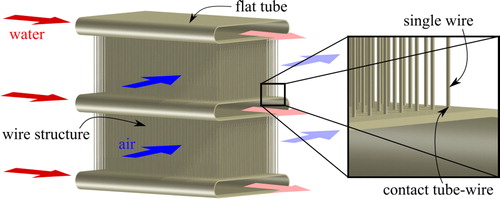
Figure 2. Different wire structure heat exchangers with high aspect ratio tested for thermal–hydraulic performance: (a) continuous wire structure; (b) pin fin structure; and (c) woven wire structure (adopted from [18,21,22]).

Figure 3. Cross-section through a wire structure heat exchanger.

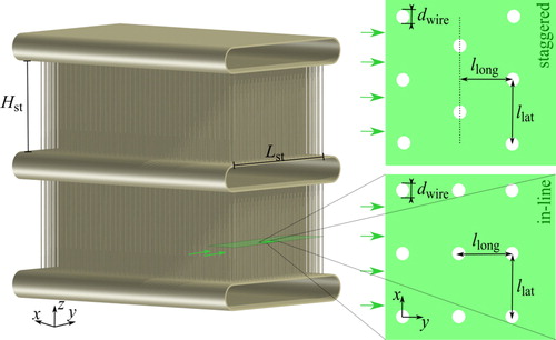
Figure 4. Boundary conditions of the in-line (a) and staggered (b) cross-section model [18].

Table 1. Definition of nondimensional input parameters to simulation model with minimal and maximal values in parametric study.

Symbol	Definition	Description	Min.	Max.
$a$	$\frac{l_{\text{lat}}}{d_{\text{wire}}}$	Nondimensional lateral distance of the wires	2	12
$b$	$\frac{l_{\text{long}}}{d_{\text{wire}}}$	Nondimensional longitudinal distance of the wires	1.3	8
${\text{Re}}_{\text{air},\mathrm{s}\mathrm{t}}$	$\frac{v_{\text{air},\mathrm{i}\mathrm{n},\mathrm{s}\mathrm{t}}{\mathrm{ }d}_{\text{wire}}\mathrm{ }{\rho }_{\text{air}}}{{\mu }_{\text{air}}\mathrm{ }}$	Reynolds number	3	60
$n_{\text{wires}}$	$\frac{L_{\text{st}}}{l_{\text{long}}}\mathrm{ }$	Number of wires in flow direction	2	200
${\text{Pr}}_{\text{air}}\mathrm{ }$	$\frac{v_{\text{air},\mathrm{i}\mathrm{n},\mathrm{s}\mathrm{t}}{c}_{p,\text{air }}{\rho }_{\text{air}}}{k_{\text{air}}}$	Prandtl number	0.71	0.71

Figure 5. Meshing of 2D cross-section with different levels of grid refinement.

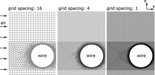
Table 2. Grid Convergence Index (GCI) based on Richardson method [27] for Nusselt number and friction factor.

Solution	$r_{\text{mesh}}$	$p_{\text{mesh}}$	${\text{GCI}}_{12}$ in %	${\text{GCI}}_{23}$ in %
Nusselt number	4	0.245	0.032	0.045
Friction factor	4	1.013	0.009	0.038

Geometry consists of five wires in row ($a$ = 8, $b$ = 3) at ${\text{Re}}_{\text{st}}$ = 11.25. Index 1 represents finer mesh, index 3 coarser mesh.

Figure 6. Pressure difference, velocity, and temperature of a 2D in-line wire structure simulation with $a$ = 10, $b$ = 3, ${\text{Re}}_{\text{st}}$ = 20, and$\mathrm{ }{n}_{\text{wires}}=20$. Contour lines for pressure difference are equally distributed. Velocity streamlines are colored based on the temperature scale.

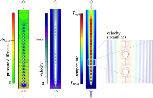
Figure 7. Nusselt number and Fanning friction factor of an in-line wire structure for a developed flow as a function of Reynolds number and geometry parameters $a$ and $b$.

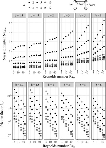
Figure 8. Correlated global (solid line) and local (dashed line) Nusselt number, ${\text{Nu}}_{\text{st}}$ and ${\text{Nu}}_{\mathrm{s}\mathrm{t},\text{local}}$, respectively, for an in-line wire arrangement, as a function of the number of wires based on the simulated global data points (squares) for ${\text{Nu}}_{\text{st}}$ and fixed values for$\mathrm{ }a=10,b=3,{\text{Re}}_{\text{st}}=20$. Downstream of the thermal entrance length (dotted line), the flow is declared as thermally developed.

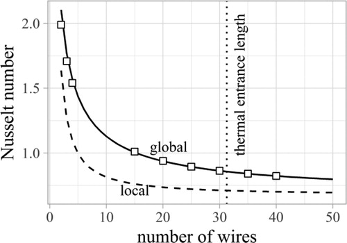
Figure 9. Correlated global (solid line) and local (dashed line) friction factor,$\mathrm{ }{\mathrm{f}}_{\text{st}}$ and ${\mathrm{f}}_{\mathrm{s}\mathrm{t},\text{local}}$, respectively, for an in-line wire arrangement as a function of the number of wires based on the simulated global data points (squares) for ${\mathrm{f}}_{\text{st}}$ and fixed values for$\mathrm{ }a=10,b=3,{\text{Re}}_{\text{st}}=20$. Downstream of hydraulic entrance length (dotted line), the flow is declared as hydraulically developed; in-line arrangement.

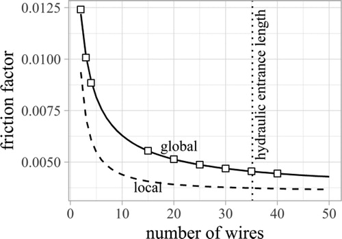
Figure 10. Predicted (correlated) values versus simulated values for (a) the Nusselt number ${\text{Nu}}_{\mathrm{s}\mathrm{t},y^{\mathrm{*}}}$ and (b) the Fanning friction factor $f_{\mathrm{s}\mathrm{t},y^{\mathrm{*}}}$. Data are based on Eqs. (13)(13) $${\text{Nu}}_{\mathrm{s}\mathrm{t},y^{\mathrm{*}}}=\mathrm{N}{\mathrm{u}}_{\mathrm{s}\mathrm{t},\mathrm{\infty }}+\frac{C_{1,\mathrm{N}\mathrm{u}}}{C_{2,\mathrm{N}\mathrm{u}}{(y}^{\mathrm{*}}-1)}\left(1-{y^{\mathrm{*}}}^{{-C}_{2,\mathrm{N}\mathrm{u}}}\right)\mathrm{ }$$(13) and (19)(19) $$f_{\mathrm{s}\mathrm{t},y^{\mathrm{*}}}=f_{\mathrm{s}\mathrm{t},\mathrm{\infty }}+\frac{C_{1,f}}{C_{2,f}{(y}^{\mathrm{*}}-1)}\left(1-{y^{\mathrm{*}}}^{{-C}_{2,f}}\right)\mathrm{ }$$(19) . The predicted values are correlated via the number of wires $n_{\text{wires}}$ (see Table 1) for specific Reynolds numbers ${\text{Re}}_{\text{st}}$ and geometry parameters $a$ and $b$ for an in-line arrangement.

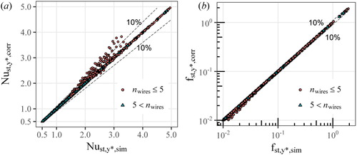
Table 3. Derived correlations for $\mathrm{N}{\mathrm{u}}_{\mathrm{s}\mathrm{t},\mathrm{\infty }}$ and ${\mathrm{f}}_{\mathrm{s}\mathrm{t},\mathrm{\infty }}$ for an in-line wire structure.

Coefficients	Auxiliary coefficients
$\mathrm{N}{\mathrm{u}}_{\mathrm{s}\mathrm{t},\mathrm{\infty }}={\tilde{A}}_{\text{Nu}}+0.021\mathrm{ }{\text{Re}}_{\text{st}}^{{\tilde{B}}_{\text{Nu}}}$	${\tilde{A}}_{\text{Nu}}=\mathrm{ }\frac{2.16\mathrm{ }b}{a\mathrm{ }+\mathrm{ }b\mathrm{ }-\mathrm{ }{\left(\frac{7.68\mathrm{ }b}{{\left(3.56\mathrm{ }+\mathrm{ }b\right)}^{0.5}}\right)}^{0.5}}$ ${\tilde{B}}_{\text{Nu}}=\frac{b^{0.345}}{\text{exp}\left(0.25\mathrm{ }a\right)\mathrm{ }}$
$f_{\mathrm{s}\mathrm{t},\mathrm{\infty }}=\text{exp}\left({\tilde{A}}_f+{\tilde{B}}_f\log \left(\mathrm{R}{\mathrm{e}}_{\text{st}}\right)\right)$	${\tilde{A}}_f=0.005531\mathrm{ }a\mathrm{ }b\mathrm{ }+\mathrm{ }0.005751\mathrm{ }{a}^2\mathrm{ }+\frac{8.6054\mathrm{ }-\mathrm{ }0.2222\mathrm{ }b}{a\mathrm{ }+\mathrm{ }0.1311\mathrm{ }a\mathrm{ }b}\mathrm{ }-\mathrm{ }0.9024\mathrm{ }-\mathrm{ }0.2985\mathrm{ }a\mathrm{ }-0.008528\mathrm{ }{b}^2$ ${\tilde{B}}_f=0.07776\mathrm{ }b\mathrm{ }+\mathrm{ }0.01624\mathrm{ }a\mathrm{ }+\mathrm{ }0.0001427\mathrm{ }a\mathrm{ }{b}^2\mathrm{ }-0.06345\mathrm{ }\log \left(a\right)-0.03442b\log \left(a\right)-1.02134$

Table 4. Derived correlations for coefficients of ${\text{Nu}}_{\text{st}}$ and ${\mathrm{f}}_{\text{st}}$ for in-line wire structure based on the Eqs. (13)(13) $${\text{Nu}}_{\mathrm{s}\mathrm{t},y^{\mathrm{*}}}=\mathrm{N}{\mathrm{u}}_{\mathrm{s}\mathrm{t},\mathrm{\infty }}+\frac{C_{1,\mathrm{N}\mathrm{u}}}{C_{2,\mathrm{N}\mathrm{u}}{(y}^{\mathrm{*}}-1)}\left(1-{y^{\mathrm{*}}}^{{-C}_{2,\mathrm{N}\mathrm{u}}}\right)\mathrm{ }$$(13) and (19)(19) $$f_{\mathrm{s}\mathrm{t},y^{\mathrm{*}}}=f_{\mathrm{s}\mathrm{t},\mathrm{\infty }}+\frac{C_{1,f}}{C_{2,f}{(y}^{\mathrm{*}}-1)}\left(1-{y^{\mathrm{*}}}^{{-C}_{2,f}}\right)\mathrm{ }$$(19) .

Coefficients	Auxiliary coefficients
$C_{1,\mathrm{N}\mathrm{u}}=\mathrm{ }\begin{array}{c}{\tilde{A}}_{1,\mathrm{N}\mathrm{u}}\text{ if }{\text{Re}}_{\text{st}}^{0.8}{a}^{2.0}{b}^{-1.1}>24\\ 0\text{ if }{\text{Re}}_{\text{st}}^{0.8}{a}^{2.0}{b}^{-1.1}\le 24\end{array}$	${\tilde{A}}_{1,\mathrm{N}\mathrm{u}}=1.6896\mathrm{ }+\mathrm{ }0.03636\mathrm{ }b\mathrm{ }+\mathrm{ }0.02745\mathrm{ }\mathrm{R}{\mathrm{e}}_{\text{st}}+\mathrm{ }\frac{0.5171\mathrm{ }a\mathrm{ }\mathrm{N}{\mathrm{u}}_{\mathrm{s}\mathrm{t},\mathrm{\infty }}}{b}\mathrm{ }+\mathrm{ }\frac{-4.4822}{2.0963\mathrm{ }+\mathrm{ }0.1266\mathrm{ }\mathrm{R}{\mathrm{e}}_{\text{st}}}\mathrm{ }-\mathrm{ }0.6369\mathrm{ }\mathrm{N}{\mathrm{u}}_{\mathrm{s}\mathrm{t},\mathrm{\infty }}$
$C_{1,f}=\mathrm{ }\begin{array}{c}{\tilde{A}}_{1,f}\text{ if }R{e}_{st}^{0.8}{a}^{1.8}{b}^{-1.0}>12\\ 0\text{ if }R{e}_{st}^{0.8}{a}^{1.8}{b}^{-1.0}\le 12\end{array}$	${\tilde{A}}_{1,f}=2.9\cdot {10}^{-5}\mathrm{ }-\mathrm{ }0.428\mathrm{ }{f}_{\mathrm{s}\mathrm{t},\mathrm{\infty }}\mathrm{ }+\frac{f_{\mathrm{s}\mathrm{t},\mathrm{\infty }}^{0.5}}{{\tilde{B}}_{1,f}}$ ${\tilde{B}}_{1,f}=1.631\mathrm{ }b\mathrm{ }+\mathrm{ }0.064\mathrm{ }a\text{ log}\left(\mathrm{R}{\mathrm{e}}_{\text{st}}\right)\mathrm{ }-\mathrm{ }0.62\mathrm{ }-\mathrm{ }0.0562\mathrm{ }a\mathrm{ }{b}^{0.5}-\mathrm{ }0.155\mathrm{ }b\text{ log}\left(\mathrm{R}{\mathrm{e}}_{\text{st}}\right)$
$C_2={\mathrm{C}}_{2,f}=C_{2,\mathrm{N}\mathrm{u}}=\frac{1}{1+{\tilde{A}}_2}$	${\tilde{A}}_2=3.77\cdot {10}^{-6}\mathrm{ }{\text{Re}}_{\text{st}}^{1.95}\mathrm{ }{a}^{3.81}\mathrm{ }{b}^{-0.68}$

Figure 11. Auxiliary coefficients$\mathrm{ }{\tilde{A}}_{\text{Nu}}\mathrm{ }$(a), ${\tilde{B}}_{\text{Nu}}$ (b), ${\tilde{A}}_f$ (c), and ${\tilde{B}}_f$ (d) needed for calculation of correlated Nusselt number and friction factor based on Table 3 for in-line arrangement. Geometry parameter $a$ is shown on the contour lines.

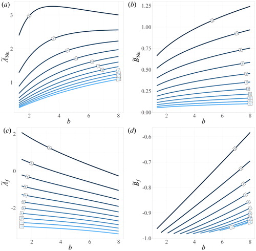
Figure 12. Nondimensional entrance lengths $L_{\text{th}}^{\mathrm{*}}$ and $L_{\text{hy}}^{\mathrm{*}}\mathrm{ }$for an in-line arrangement based on the Reynolds number ${\text{Re}}_{\text{st}}$ and geometry parameters $a$ and $b$. Entrances lengths below 0.1 are not shown.

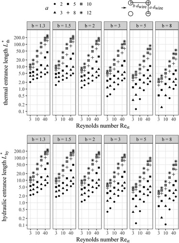
Figure 13. Predicted (correlated) values versus simulated values for (a) the Nusselt number ${\text{Nu}}_{\mathrm{s}\mathrm{t},\mathrm{\infty }}$ and (b) the Fanning friction factor ${\mathrm{f}}_{\mathrm{s}\mathrm{t},\mathrm{\infty }}$ for a developed flow. Data are based on Table 3. The predicted values are correlated via the Reynolds number ${\text{Re}}_{\text{st}}$ and geometry parameters $a$ and $b$ for an in-line wire arrangement.

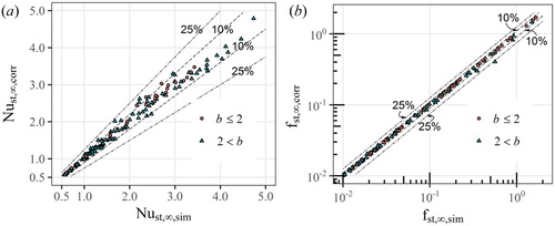
Figure 14. Predicted (correlated) values versus simulated values for (a) the Nusselt number ${\text{Nu}}_{\mathrm{s}\mathrm{t},{\mathrm{y}}^{\mathrm{*}}}$ and (b) the Fanning friction factor ${\mathrm{f}}_{\mathrm{s}\mathrm{t},y^{\mathrm{*}}}$. Data are based on Eqs. (13)(13) $${\text{Nu}}_{\mathrm{s}\mathrm{t},y^{\mathrm{*}}}=\mathrm{N}{\mathrm{u}}_{\mathrm{s}\mathrm{t},\mathrm{\infty }}+\frac{C_{1,\mathrm{N}\mathrm{u}}}{C_{2,\mathrm{N}\mathrm{u}}{(y}^{\mathrm{*}}-1)}\left(1-{y^{\mathrm{*}}}^{{-C}_{2,\mathrm{N}\mathrm{u}}}\right)\mathrm{ }$$(13) and (19)(19) $$f_{\mathrm{s}\mathrm{t},y^{\mathrm{*}}}=f_{\mathrm{s}\mathrm{t},\mathrm{\infty }}+\frac{C_{1,f}}{C_{2,f}{(y}^{\mathrm{*}}-1)}\left(1-{y^{\mathrm{*}}}^{{-C}_{2,f}}\right)\mathrm{ }$$(19) (Tables 3 and 4). The predicted values are correlated via the Reynolds number ${\text{Re}}_{\text{st}}$, geometry parameters $a$ and $b$, and the number of wires for an in-line wire arrangement.

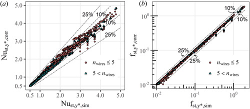
Table 5. Percentage of correlated data which satisfy a relative residual error below 5% and 10% for ${\text{Nu}}_{\mathrm{s}\mathrm{t},\mathrm{\infty }}$, ${\mathrm{f}}_{\mathrm{s}\mathrm{t},\mathrm{\infty }}$,$\mathrm{ }{\text{Nu}}_{\mathrm{s}\mathrm{t},{\mathrm{y}}^{\mathrm{*}}}$, and ${\mathrm{f}}_{\mathrm{s}\mathrm{t},{\mathrm{y}}^{\mathrm{*}}}$.

		${\text{Nu}}_{\mathrm{s}\mathrm{t},\mathrm{\infty }}$	$f_{\mathrm{s}\mathrm{t},\mathrm{\infty }}$	${\text{Nu}}_{\mathrm{s}\mathrm{t},{\mathrm{y}}^{\mathrm{*}}}$		$f_{\mathrm{s}\mathrm{t},y^{\mathrm{*}}}$
		$n_{\text{wires}}$
		$>L_{\text{th}}^{\mathrm{*}}$	$>L_{\text{hy}}^{\mathrm{*}}$	$>2$	> 5	> 2	> 5
Relative residual error	<5%	81 %	94 %	76 %	79 %	89 %	92 %
	<10%	94 %	99 %	93 %	95 %	97 %	99 %

The percentage is specified for different number of wires in an in-line wire arrangement.

Table B1. Predicted correlation for coefficients of ${\text{Nu}}_{\text{st}}$ and ${\mathrm{f}}_{\text{st}}$ for staggered wire structure based on the Eqs. (13)(13) $${\text{Nu}}_{\mathrm{s}\mathrm{t},y^{\mathrm{*}}}=\mathrm{N}{\mathrm{u}}_{\mathrm{s}\mathrm{t},\mathrm{\infty }}+\frac{C_{1,\mathrm{N}\mathrm{u}}}{C_{2,\mathrm{N}\mathrm{u}}{(y}^{\mathrm{*}}-1)}\left(1-{y^{\mathrm{*}}}^{{-C}_{2,\mathrm{N}\mathrm{u}}}\right)\mathrm{ }$$(13) and (19)(19) $$f_{\mathrm{s}\mathrm{t},y^{\mathrm{*}}}=f_{\mathrm{s}\mathrm{t},\mathrm{\infty }}+\frac{C_{1,f}}{C_{2,f}{(y}^{\mathrm{*}}-1)}\left(1-{y^{\mathrm{*}}}^{{-C}_{2,f}}\right)\mathrm{ }$$(19) .

Coefficients	Auxiliary coefficients
${\text{Nu}}_{\mathrm{s}\mathrm{t},\mathrm{\infty }}={\tilde{A}}_{\text{Nu}}+0.021\mathrm{ }{\text{Re}}_{\text{st}}^{{\tilde{B}}_{\text{Nu}}}$	${\tilde{A}}_{\text{Nu}}=\mathrm{ }0.91\mathrm{ }+\frac{2.57}{b}\mathrm{ }+\mathrm{ }\frac{2.2\mathrm{ }-\mathrm{ }0.78a}{\text{exp}\left(b\right)}$ ${\tilde{B}}_{\text{Nu}}=0.598\mathrm{ }+\mathrm{ }0.065\mathrm{ }\frac{a}{b}\mathrm{ }-\mathrm{ }0.393{\left(\frac{a}{b}\right)}^{0.5}$
$f_{\mathrm{s}\mathrm{t},\mathrm{\infty }}=\text{exp}\left({\tilde{A}}_f+{\tilde{B}}_f\log \left(\mathrm{R}{\mathrm{e}}_{\text{st}}\right)\right)$	${\tilde{A}}_f=1.28\mathrm{ }+\mathrm{ }0.62\mathrm{ }\frac{b}{a}\mathrm{ }+\frac{4.31\mathrm{ }-\mathrm{ }2.05\mathrm{ }{\left(a\right)}^{0.5}}{b}\mathrm{ }-\mathrm{ }0.015\mathrm{ }a\mathrm{ }-\mathrm{ }2.06\text{ log}\left(b\right)$ ${\tilde{B}}_f=-\frac{1.43}{b}\mathrm{ }+\frac{2.65}{a\mathrm{ }b}\mathrm{ }+\mathrm{ }0.078\frac{a}{b^2}\mathrm{ }-\mathrm{ }0.297\mathrm{ }-\mathrm{ }b\mathrm{ }{0.23}^a\mathrm{ }-\mathrm{ }0.025\mathrm{ }a$
$C_{1,\mathrm{N}\mathrm{u}}=\mathrm{ }\begin{array}{ll}{\tilde{A}}_{1,\mathrm{N}\mathrm{u}}& \text{if }{\text{Re}}_{\text{st}}^{0.9}{a}^{2.4}{b}^{-1.2}>240\\ 0& \text{if }{\text{Re}}_{\text{st}}^{0.9}{a}^{2.4}{b}^{-1.2}\le 240\end{array}$	${\tilde{A}}_{1,\mathrm{N}\mathrm{u}}=0.22\mathrm{ }+\mathrm{ }0.16\mathrm{ }\mathrm{R}{\mathrm{e}}_{\text{st}}+\frac{0.89}{b}+\mathrm{ }0.02\mathrm{ }a\mathrm{ }b\mathrm{ }+\mathrm{ }0.000045\mathrm{ }\mathrm{R}{\mathrm{e}}_{\text{st}}^3-\mathrm{ }0.35\mathrm{ }b\mathrm{ }-\mathrm{ }0.0021\mathrm{ }\mathrm{R}{\mathrm{e}}_{\text{st}}^2-\mathrm{ }0.2{\text{ Nu}}_{\mathrm{s}\mathrm{t},\mathrm{\infty }}^2$
$C_{1,f}=\mathrm{ }\begin{array}{cc}{\tilde{A}}_{1,\mathrm{f}}& \text{if }\mathrm{R}{\mathrm{e}}_{st}^{0.9}{a}^{2.2}{b}^{-1.1}>255\\ 0& \text{if }\mathrm{R}{\mathrm{e}}_{\mathrm{s}\mathrm{t}}^{0.9}{a}^{2.2}{b}^{-1.1}\le 255\end{array}$	${\tilde{A}}_{1,f}=f_{\mathrm{s}\mathrm{t},\mathrm{\infty }}\mathrm{ }\left[0.15\mathrm{ }\mathrm{R}{\mathrm{e}}_{\text{st}}^{0.5}-\frac{4.97}{a}\mathrm{ }+\mathrm{ }\frac{0.017\mathrm{ }a{\mathrm{ }\left(0.87\mathrm{ }+\mathrm{ }\mathrm{R}{\mathrm{e}}_{\text{st}}\right)}^{0.5}{\left(13.85\text{ log}\left(a\right)\right)}^{0.5}}{b}\mathrm{ }-\mathrm{ }0.46\right]\mathrm{ }$
$C_{2,\mathrm{N}\mathrm{u}}=\mathrm{ }\frac{1.20}{1+{\tilde{A}}_{2,\mathrm{N}\mathrm{u}}}$	${\tilde{A}}_{2,\mathrm{N}\mathrm{u}}=3.070\cdot {10}^{-4}\mathrm{ }{\text{Re}}_{\text{st}}^{0.886}\mathrm{ }{a}^{2.719}\mathrm{ }{b}^{-0.928}$
$C_{2,f}=\mathrm{ }\frac{1.01}{1+{\tilde{A}}_{2,f}}$	${\tilde{A}}_{2,f}=3.286\cdot {10}^{-6}\mathrm{ }{\text{Re}}_{\text{st}}^{1.448}\mathrm{ }{a}^{3.842}\mathrm{ }{b}^{-1.260}$

Correlation is valid for:$\mathrm{ }3\le a\le 12$,$\mathrm{ }1.3\le b\le 8$,$\text{ and }3\le \mathrm{R}{\mathrm{e}}_{\text{st}}\le 60$.

Table B2. Percentage of correlated data which satisfy a relative residual error below 5% and 10% for ${\text{Nu}}_{\mathrm{s}\mathrm{t},\mathrm{\infty }}$, ${\mathrm{f}}_{\mathrm{s}\mathrm{t},\mathrm{\infty }}$,$\mathrm{ }{\text{Nu}}_{\mathrm{s}\mathrm{t},{\mathrm{y}}^{\mathrm{*}}}$, and ${\mathrm{f}}_{\mathrm{s}\mathrm{t},{\mathrm{y}}^{\mathrm{*}}}\mathrm{ }$in staggered wire arrangement.

		${\text{Nu}}_{\mathrm{s}\mathrm{t},\mathrm{\infty }}$	$f_{\mathrm{s}\mathrm{t},\mathrm{\infty }}$	${\text{Nu}}_{\mathrm{s}\mathrm{t},{\mathrm{y}}^{\mathrm{*}}}$		$f_{\mathrm{s}\mathrm{t},y^{\mathrm{*}}}$
		$n_{\text{wires}}$
		$>L_{\text{th}}^{\mathrm{*}}$	$>L_{\text{hy}}^{\mathrm{*}}$	$>2$	> 5	> 2	> 5
Relative residual error $3\le a\le 12$	<5%	67	71	68	68	68	69
	<10%	90	89	92	91	87	88
Relative residual error $5\le a\le 12$	<5%	70	80	73	74	78	79
	<10%	88	95	91	90	95	95

The percentage is specified for different number of wires. Correlation is valid for: $3\le a\le 12$, $1.3\le b\le 8$, and $3\le \mathrm{R}{\mathrm{e}}_{\text{st}}\le 60$.

H. Fugmann, P. D. Lauro, and L. Schnabel, Heat Transfer Surface Area Enlargement by Usage of Metal Textile Structures – Development, Potential and Evaluation. Dresden: International Textile Conference, 2016. DOI: 10.3390/en10091341.

 Google Scholar

H. Fugmann, P. Di Lauro, A. Sawant, and L. Schnabel, “Development of heat transfer surface area enhancements: A test facility for new heat exchanger designs,” Energies, vol. 11, no. 5, pp. 1322, 2018. DOI: 10.3390/en11051322.

 Web of Science ®Google Scholar

MinWaterCSP Project, Cooling Systems: Wire structure heat transfer surfaces. MinWaterCSP consortium. Available: https://www.minwatercsp.eu/technologies/cooling-systems/.

 Google Scholar

I. B. Celik, U. Ghia, P. J. Roache, C. J. Freitas, H. Coleman, and P. E. Raad, “Procedure for Estimation and Reporting of Uncertainty Due to Discretization in CFD Applications,” J. Fluids Eng., vol. 130, pp. 078001 (1–4) 2008. DOI: 10.1115/1.2960953.

 Google Scholar