A two-level machine learning approach for predicting thermal striping in T-junctions with upstream elbow

Figures & data

Figure 1. Schematic of the T-junction flow configuration with upstream elbow.

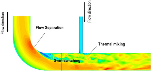
Table 1. The geometry of the elbow tee configuration.

	Main	Branch
Mass flow rate ($\mathit{\text{kg}}/s)$	${\dot{m}}_c=$63.32 ∼ 601.3	${\dot{m}}_h=$0.65 ∼ 5.65
Temperature ($\mathrm{°C})$	$T_c=$40	$T_h=$240
Diameter (mm)	$D_m=$387.35	$D_b=$49.48
Elbow radius of curvature (mm)	$R_c=$542.29
Distance between bend and junction (mm)	$L=$774.7

Figure 2. Nonlinear interpolation of bias based on parametric distance. For a given mode index $\mathit{m}$ and an input parameter vector $\mathit{\mu },$ the reference mode ${\mathit{\varphi }}_m\left({\mathit{\mu }}^{\left(\mathit{*}\right)}\right)$ is obtained from the structure predictor. The term ${\mathit{ϵ}}_{\mathit{m}}\left(\mathit{\mu },{\mathit{\mu }}^{\left(\mathit{*}\right)}\right)$ is the approximation bias between two different inputs ${\mathit{ϵ}}_{\mathit{m}}\left(\mathit{\mu },{\mathit{\mu }}^{\left(\mathit{*}\right)}\right)={\mathit{\varphi }}_m\left(\mathit{\mu }\right)-{\mathit{\varphi }}_m\left({\mathit{\mu }}^{\left(\mathit{*}\right)}\right);\mathit{d}\left(\mathit{\mu },{\mathit{\mu }}^{\left(\mathit{*}\right)}\right)=\Vert \mathit{\mu }-{\mathit{\mu }}^{\mathit{*}}\Vert$ is the parametric distance.

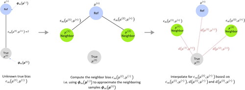
Figure 3. Training workflow of the machine learning framework: (a) Structure Predictor: Gradient Boosting; (b) Structure corrector: Parameterized CNN.

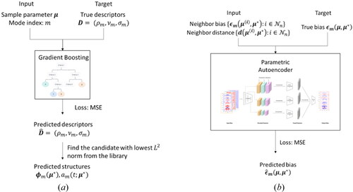
Figure 4. Prediction workflow of the two-machine framework.

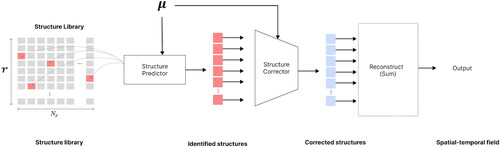
Figure 5. Design of experiment in terms of mass flux ratio, which corresponds to different power levels in a reactor operation.

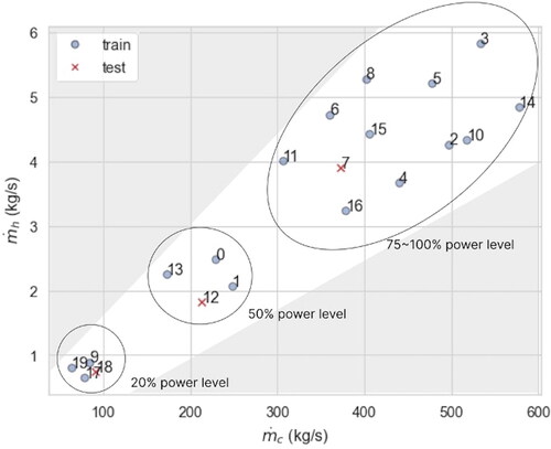
Figure 6. Illustration of data acquisition points. A total of 576 equally spaced probes are placed at the top region of the pipe to collect the flow snapshots from the high-fidelity simulations.

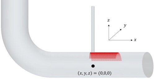
Figure 7. Schematics of the POD-mirroring. The data from the reduced data domain ($+y$ plane) is used to extract POD structures. The resulting spatial modes are mirrored to the $-y$ plane for imposing flow symmetry.

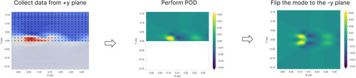
Figure 8. Flow snapshots of streamwise velocity. For different mass flow rates, the results show high nonlinearity.

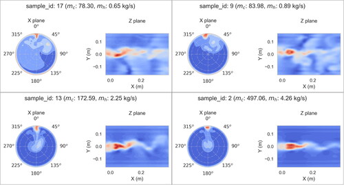
Figure 9. Two main types of vortical structures were obtained from performing POD on the full data window: (a) large, elongated vortices observed in low mass flow rate cases (sample 17) (b) von Karman vortex street type of vortices observed in high mass flow rate cases (sample 2).

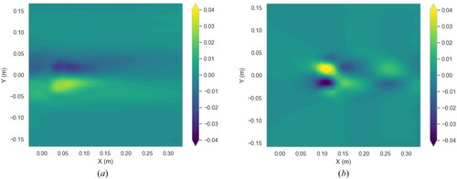
Figure 10. The first POD mode obtained from the reduced data window. (a) sample 17 (b) sample 2. The same vortical structures are obtained when comparing with Figure 9.

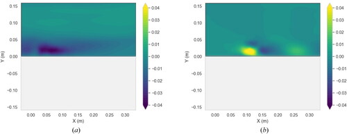
Figure 11. The oscillatory characteristics of turbulence structures under different power levels but with the same mass flux ratio (∼40). (a) spatial modes. (b) Power spectrum density (PSD) for the temporal coefficients (unit: $m^2/s^2\mathit{\text{ Hz }}).$ In this example, sample 17 corresponds to the operating condition at 20% power level, whereas sample 2 represents the scenario at 100% power level.

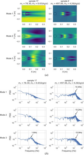
Figure 12. Flow structures deformation with slight parameter variations: (a) velocity field (b) temperature field. The presented samples depict flow conditions at approximately 50% power levels.

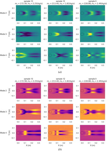
Figure 13. Assessment of the structure predictor for velocity POD modes: (a) sample 7 (b) sample 0 (c) sample 9. The first row shows the temporal coefficients of the POD modes (in frequency domain). The second and third rows show the true and predicted structures, respectively.

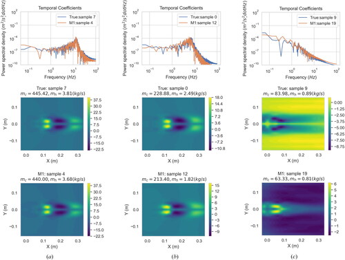
Figure 14. Assessment of the structure predictor for temperature POD modes: (a) sample 7 (b) sample 0 (c) sample 9. The first row shows the temporal coefficients of the POD modes (in frequency domain). The second and third rows show the true and predicted structures, respectively.

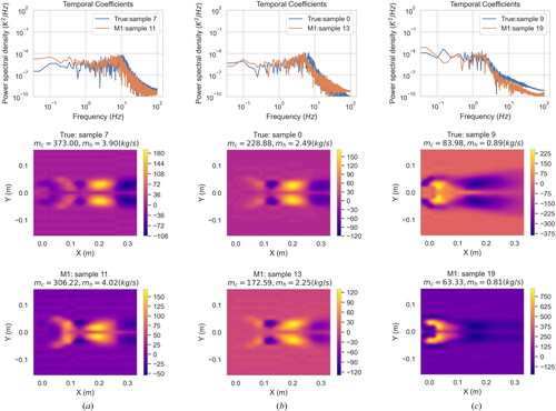
Figure 15. Results of bias prediction: velocity (a) training: sample 11, mode 1 (b) Testing: sample 7, mode 1. The term true bias refers to the bias that arises when using the reference structures to approximate the true structures (i.e. ${\mathit{ϵ}}_m\left(\mathit{\mu },{\mathit{\mu }}^{*}\right)$); the predicted bias represents the M2 prediction (i.e. ${\widehat{\mathit{ϵ}}}_m\left(\mathit{\mu },{\mathit{\mu }}^{*}\right)$).

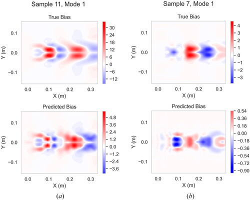
Figure 16. Results of bias prediction: temperature (a) training sample 11, mode 1 (b) testing: sample 7, mode 1. The term true bias refers to the bias that arises when using the reference structures to approximate the true structures (i.e. ${\mathit{ϵ}}_m\left(\mathit{\mu },{\mathit{\mu }}^{*}\right)$); the predicted bias represents the M2 prediction (i.e. ${\widehat{\mathit{ϵ}}}_m\left(\mathit{\mu },{\mathit{\mu }}^{*}\right)$).

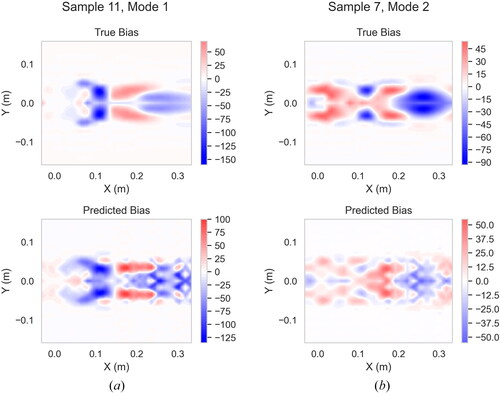
Figure 17. Field RMS prediction (a) $u_{\mathit{\text{rms}}}$ (b) $T_{\mathit{\text{rms}}}.$ The term “M1” refers to using structure predictor only; the term “M1 + M2” refers to using both structure predictor and structure corrector.

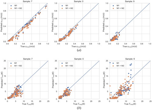
Figure 18. Emulation of velocity field. Signals with peak $u_{\mathit{\text{rms}}}$ magnitudes are presented. (a) sample 7 (b) sample 0 (c) sample 9 (Left: the probe location; the coloring indicates the $u_{\mathit{\text{rms}}}$ magnitude. Right: power spectrum density of the true/emulated velocity signals).

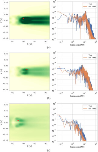
Figure 19. Emulation of temperature field. Signals with peak $T_{\mathit{\text{rms}}}$ magnitudes are presented. (a) sample 7 (b) sample 0 (c) sample 9 (Left: the probe location (Left: the probe location; the coloring indicates the $T_{\mathit{\text{rms}}}$ magnitude. Right: power spectrum density of the true/emulated velocity signals).

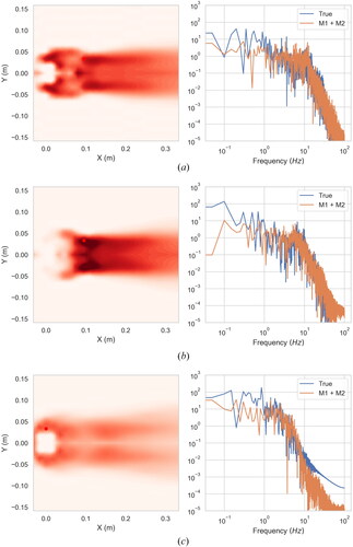
Table 2. Computational times for the full-model CFD simulation (single processor) and the framework surrogate.

	Training time	Runtime
Full model	8,840 hr^1	442 hr (one full simulation)
Two-machine framework surrogate	Structure predictor: 11.8 ($s$) Structure corrector: 149$(\mathrm{\text{min}})$	0.78 ($s)$
Runtime Acceleration (Full-model / surrogate)-		7.57 E + 7

¹ Time for generating the training data (20 samples).