Interventional probability of causation (IPoC) with epidemiological and partial mechanistic evidence: benzene vs. formaldehyde and acute myeloid leukemia (AML)

Figures & data

Figure 1. A Simple causal Bayesian network (BN).

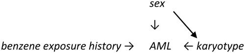
Figure 2. A Modified causal network with genotype as a common cause of sex and karyotype.

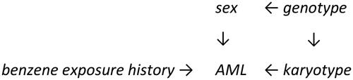
Table 1. Example of a hypothetical CPT.

Benzene exposure history	Karyotype	P(AML = 1 | Pa(AML))
Non-occupational	Non-susceptible	0.001
Non-occupational	Susceptible	0.006
Occupational	Non-susceptible	0.001
Occupational	Susceptible	0.009

Table 2. Example of a hypothetical causal CPT.

Sex	Benzene exposure history	Karyotype	P(AML = 1 | Pa(AML))
M	Non-occupational	Non-susceptible	0.0005
M	Non-occupational	Susceptible	0.0055
M	Occupational	Non-susceptible	0.0005
M	Occupational	Susceptible	0.0085
F	Non-occupational	Non-susceptible	0.0015
F	Non-occupational	Susceptible	0.0065
F	Occupational	Non-susceptible	0.0015
F	Occupational	Susceptible	0.0095

Table 3. Some popular Bayesian network (BN) inference algorithms.

Methods	Main ideas	Comments and references
Junction Trees	Convert Bayesian network to a tree-like structure and propagate probabilities to infer marginal distributions.	Computationally intensive for large networks. Require triangulation, leading to potential inefficiency. Reference: Lauritzen and Spiegelhalter (1988)
Variable Elimination algorithms	Systematically eliminate variables by summing conditional probabilities over their values (“marginalizing them out”). Reduce complexity by focusing on query and evidence variables.	Assumptions: Can be computationally expensive. Sequence of elimination affects efficiency. References: Zhang and Poole (1996); Dechter (1999) for efficient “bucket elimination”
Arc-Reversal (Hugin algorithm)	Use Bayes’ rule to reverse the directions of arcs to reduce the size of the problem, potentially making inference more efficient.	Like other exact methods, it can be computationally challenging for large networks. Efficiency gains depend on the structure of the network. Reference: Andersen et al. (1989)
Recursive Conditioning	Breaks the network down into smaller pieces recursively and solves them.	More memory-efficient than methods like Junction Trees. Reference: Darwiche (2001)
Clique Tree Calibration	Represents the Bayesian network using a clique tree and then calibrates it to perform inference.	Computationally challenging for large networks. Reference: Koller and Friedman 2009
Message Passing Algorithms	Pass messages (probability distributions) between nodes of the network to determine the marginal distributions.	Require a tree-structured graph or must be transformed into one. Can be inefficient for certain structures. References: Pearl (1988); Shafer and Shenoy (1990)

Figure 3. A Simplified hypothetical example Bayesian network model.

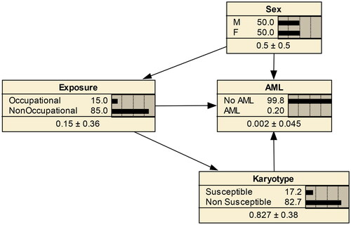
Figure 4. Conditional probabilities of AML with (right) and without (left) occupational exposure.

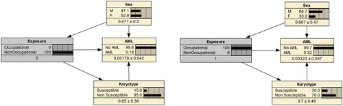
Figure 5. Conditional probabilities of AM with (right) and without (left) occupational exposure, for men (top) and women (bottom).

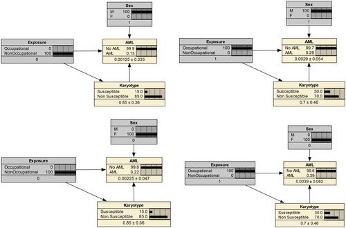
Table 4. Example of qualitative exposure levels defined by the qualitatively different responses elicited.

Exposure	Toxicological response profile	Target stem cell damage and cancer risk
Very low	Parent compound and any toxic metabolites are detoxified efficiently. Toxic metabolites do not reach target cells.	Background level; no incremental risk
Low	Hormesis: Toxic metabolites reach target cells. Protective resources (e.g. glutathione) are activated but not depleted or saturated (i.e. threshold is not exceeded). Some adaptive responses may be initiated, such that damage is limited or even prevented, i.e. they more than compensate for threats from toxic metabolites (i.e. hormetic response).	Damage limited or overcompensated. Hormesis response: Below-background risk Threshold response: Background risk
Medium	Some protective resources are depleted or saturated. Toxic metabolites reach target cells and damage them, perhaps causing oxidative stress, genotoxic and clastogenic damage, and chromosomal aberrations. Target cell populations maintain homeostasis by limiting and compensating for damage via changes in proliferation, apoptosis, cell defenses, (e.g. anti-oxidant production) and repair.	Graded cytotoxic response. No excess cancer risk.
High	Target cell defenses are depleted or saturated. Cells are killed via acute cytotoxicity. This can lead to compensating regenerative hyperplasia. Stem cells with genotoxic and/or epigenetic damage that are produced (“initiation”) and not repaired or removed via apoptosis proliferate via clonal expansion (“promotion”). Some may become fully malignant (“progression”) leading to in situ cancer. Those that subsequently escape immune surveillance and local control can after a latency period lead to malignancy or tumors.	Graded cytotoxic, genotoxic, clastogenic, and/or epigenetic responses; graded cancer risk
Very high	Cancerous cells are produced at maximum (saturated) rate, although cell damage might be so great that cell death occurs and cancer initiation rate flattens.	Saturated cancer risk

Table 5. Examples of multipliers and multiplier ranges.

Exposure	Toxicological response profile	Examples of Ri
Very low	Parent compound and any toxic metabolites are detoxified efficiently. Toxic metabolites do not reach target cells.	1
Low	Hormesis: Toxic metabolites reach target cells. Protective resources (e.g. glutathione) are activated but not depleted or saturated. They more than compensate for threats from toxic metabolites.	≤1
Medium	Some protective resources are depleted or saturated. Toxic metabolites reach target cells and damage them, perhaps causing oxidative stress, genotoxic and clastogenic damage, and chromosomal aberrations. Target cell populations maintain homeostasis by limiting and compensating for damage via changes in proliferation, apoptosis, cell defenses, (e.g. anti-oxidant production) and repair.	≤1
High	Target cell defenses are depleted or saturated. Cells are killed via acute cytotoxicity. This can lead to compensating regenerative hyperplasia (Ri1 > 1). Stem cells with unrepaired genotoxic and/or epigenetic damage that becomes locked in by mitosis and that escape apoptosis (“initiation,” Ri2 > 0) may proliferate via clonal expansion (“promotion,” Ri3 > 0). Some may become fully malignant (“progression,” Ri4 > 0) leading to in situ cancer. Those that subsequently escape immune surveillance and local control can cause tumors after a latency period.	1–3 for Ri1 = Ni/N0 1–4 for Ri2 = µ1i/µ10 1–2 for Ri4 = µ2i/µ20 1–2 for Ri3 = (d0 – b0)/(di − bi) 1–48 for Ri = Ri1Ri2Ri3Ri4, their product
Very high	Cancerous cells are produced at maximum (saturated) rate	≤48

Table 6. Examples of sources of inter-individual variability in epidemiological studies.

Factor	System/mechanism	Disease	Estimated measure of association	Citation
CYP1A1 MspI and exon 7	Genetic polymorphisms	Lung cancer	m-OR = 1.26 (95% CI: 1.12–1.42) for Type C m-OR = 1.20 (95% CI: 1.13–1.28) for Types B&C	Zhan et al. 2011
CYP1A1 MspI	Genetic polymorphisms	Squamous cell lung cancer	m-OR = 1.81 (1.52–2.14) for (CT + TT) vs CC allele	Ji et al. 2012
CYP1A1 MspI	Genetic polymorphisms	Small cell lung cancer	m-OR = 0.98 (0.73–1.32) for (CT + TT) vs CC allele	Ji et al. 2012
loci with gene variants: 11q13.2(rs4930561); 6p21.32 (rs3916765)	genes operating in histone methylation (KMT5B) & immune function (HLA)	Acute Myeloid Leukemia	m-OR = 1.17 (95% CI: 1.11–1.24) m-OR = 1.75 (95% CI: 1.44–2.14)	Lin et al. 2021
A allele and AA genotype of CYP2D6	Cell Damage Detection and Repair (Cytochrome P450)	Lung Cancer	Adj-OR = 1.35 (95% CI: 1.13-1.60)	Li et al. 2019
GSTM1 null genotype	phase II enzymes that protect cells from oxidative stress	Oral cancers	Pooled-OR = 1.551 (95% CI: 1.355-1.774)	Kumar et al. 2022
GSTT1 null genotype	phase II enzymes that protect cells from oxidative stress	Oral cancers	Pooled-OR = 1.377 (95% CI: 1.155–1.642)	Kumar et al. 2022
GSTM1 null genotype	phase II enzymes that protect cells from oxidative stress	Endometriosis	m-OR = 1.56 (95% CI: 1.25–1.95)	Xin et al. 2016
GSTM1 and GSTT1 null genotypes	phase II enzymes that protect cells from oxidative stress	Endometriosis	m-OR = 1.68 (95% CI: 1.29–2.17)	Xin et al. 2016
CAT (rs1001179)	Affects catalase expression and ROS detoxification	Prostate cancer	m-OR for TT vs. TC + CC = 1.39 (95%CI 1.17-1.66)	Alvarez-Gonzalez et al., 2023
LSP1 rs3817198 polymorphism	F-actin bundling protein affecting neutrophils	Breast cancer	homozygous model: m-OR= 1.18 (95% CI: 1.09–1.28) in Caucasians and Asians	Chen et al. 2022
SOD2 polymorphism (T/T + T/C vs. C/C)	Superoxide dismutase, an antioxidant enzyme	Non-Hodgkin Lymphoma	m-OR = 1.166 (95% CI: 1.017–1.336)	Kang 2015
SOD2 polymorphism (T vs. C)	Superoxide dismutase, an antioxidant enzyme	Bladder cancers	m-OR = 1.129 (95% CI: 0.971–1.312)	Kang 2015
BRCA1 mutation carriers	DNA repair proteins	Breast cancer	cumulative breast cancer risk to age 80 years = 72% (95% CI: 65%–79%)	Kuchenbaecker et al. 2017
BRCA2 mutation carriers	DNA repair proteins	Breast cancer	cumulative breast cancer risk to age 80 years = 69% (95% CI: 61%–77%)	Kuchenbaecker et al. 2017
BRCA1 mutation carriers	DNA repair proteins	Ovarian cancer	cumulative ovarian cancer risk to age 80 years = 44% (95% CI: 36%–53%)	Kuchenbaecker et al. 2017
BRCA2 mutation carriers	DNA repair proteins	Ovarian cancer	cumulative ovarian cancer risk to age 80 years = 17% (95% CI: 11%–25%)	Kuchenbaecker et al. 2017
rs1256030 variant (TT genotype	estrogen receptor b (ESR2) gene	Breast cancer	OR = 1.86 (95% CI: 1.05–3.28)	Gallegos-Arreola et al. 2022

Figure 6. Cumulative probability distribution functions (CDFs) of IPoC (left) and AS (right).

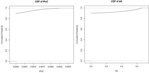
Figure 7. Example of a sensitivity analysis showing how the unconditional probability of causation, mean(AS) (which is the same as mean(CAS) if M₀ and R are the only direct causes of risk) depends on the assumed probability that exposure is too low to affect the number of malignant cells formed. Source: Code at https://chat.openai.com/share/04aa37d4-ee74-4c8a-ae64-c32e70d7fbeb.

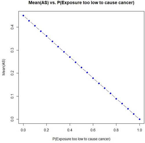
Figure 8. Decomposition of a causal exposure-response function, exposure, x → risk (bottom) into two components: exposure, x → internal dose, y (upper left); and internal dose, y → risk (upper right).

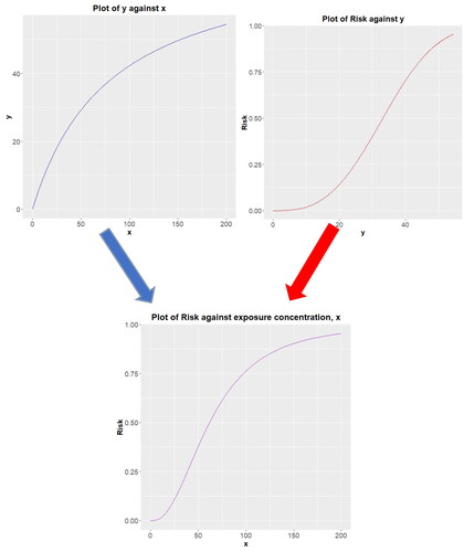
Table 7. Selected causal discovery algorithms for identifying plausible causal models from data.

Method	Main ideas	Assumptions and limitations
LinGAM (Linear Non-Gaussian Acyclic Model)	Exploits the non-Gaussian distributions of variables to infer a unique causal order by estimating linear causal effects.	Assumes linear relationships and non-Gaussian disturbances.
FCI (Fast Causal Inference)	Uses conditional independence tests to uncover causal structures, even with hidden confounders, by orienting undirected edges.	Does not always identify a unique causal model.
BackSHIFT algorithm	By analyzing how variable distributions change across different environments, it identifies which variables drive these changes.	Requires repeated measurements and assumes non-linearity in some relations.
PC Algorithm (Peter-Clark Algorithm)	Begins with a full, undirected graph and iteratively prunes edges based on conditional independence tests.	Assumes no hidden confounders.
GES (Greedy Equivalence Search)	Iteratively adds and removes arrows in the graph to find structures that best fit the data based on a scoring criterion.	Can sometimes get stuck in local optima.
CAM (Causal Additive Model)	Utilizes a non-linear, non-Gaussian framework to deduce causal relationships by separating the observed data into additive components.	Assumes each cause has an additive effect on the outcome.
TETRAD	Utilizes the concept of "vanishing tetrads", which are statistical constraints on observed data, to uncover potential causal structures. By searching for these vanishing tetrads in data, the software helps in deducing constraints that can infer potential causal connections between variables. Additionally, TETRAD allows for the integration of background knowledge and supports multiple algorithms for causal exploration.	Depending on the chosen algorithm within TETRAD, various assumptions such as faithfulness and causal sufficiency may apply. Limitations might also vary based on the specific method used.
Invariant Causal Prediction (ICP)	Identifies variables that have invariant prediction across different environments or interventions, which is indicative of a causal effect. This method leverages the fact that causal relationships remain consistent across varying conditions, while non-causal relationships may change.	Requires multiple datasets from different environments or interventions. Assumes that the causal structure remains constant across these settings, while the distributions of the variables can change.
Granger causality testing	A statistical hypothesis test used to determine whether one time series can predict another. If a variable X Granger-causes Y, past values of X should contain information that helps predict Y beyond the information contained in past values of Y alone.	Assumes linearity and stationary time series. Does not necessarily imply true causality, but rather an ability to forecast.
Directed Information Flow	Measures the amount of information that one time series (source) transfers to another (destination) considering the entire history of the system. It quantifies causal dependencies between systems in terms of their information content.	Assumes stationarity of time series. It measures causal influence in terms of information transfer, which may differ from direct causal effects.

Source: Table created with help from ChatGPT4; see https://chat.openai.com/share/196a6943-6b44-46f8-b569-b177949a3591.

Figure 9. A “no side effects” conceptualization of proposed causal pathways linking benzene exposure to AML risk. Source: McHale et al. (2012)

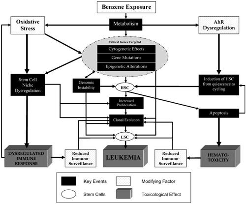
Figure 10. A Proposed causal DAG model for benzene-induced AML risk and side effects.

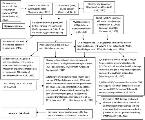
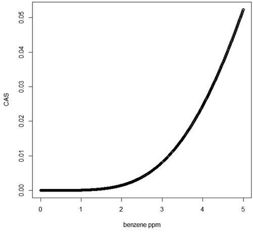
Figure 11. Plausible upper-bound estimates of IPoC as a function of benzene concentration in air. # Source: R code for left side of Figure 11. PPH = exceedance probability for PH; Y0PH = 69.5; YmaxPH = 5293; X50PH = 107.1; Y0HQ = 6.36; YmaxHQ = 376; X50HQ = 50.9; X <- (0:1000)/20; YHQ <- Y0HQ + YmaxHQ*X/(X50HQ + X); YPH <- Y0PH + YmaxPH*X/(X50PH + X); PHQ <- 1-pnorm(log(68.1), log(YHQ), log(2.24)/1.96); PPH <- 1-pnorm(log(521.5), log(YPH), log(2.24)/1.96); plot(X, PPH*1e-7, ylab = "IPoC", xlab = "benzene ppm"); # plot(X, PPH*0.54, ylab = "CAS", xlab = "benzene ppm");

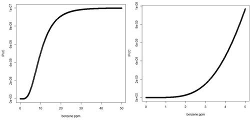
Figure 12. Plausible upper-bound estimates of causal assigned share (CAS) for AML as a function of benzene concentration in air.

Lauritzen SL, Spiegelhalter DJ. 1988. Local computations with probabilities on graphical structures and their application to expert systems. J R Stat Soc Series B Methodological. 50(2):157–194. doi: 10.1111/j.2517-6161.1988.tb01721.x.

 Google Scholar

Zhang W, Poole D. 1996. Exploiting Causal Independence in Bayesian Network Inference. jair. 5(1):301–328. doi: 10.1613/jair.305.

 Google Scholar

Dechter R. 1999. Bucket elimination: a unifying framework for reasoning. Artif Intell. 113(1–2):41–85. https://www.sciencedirect.com/science/article/pii/S0004370299000594. doi: 10.1016/S0004-3702(99)00059-4.

 Web of Science ®Google Scholar

Andersen SK, Olesen KG, Jensen FV, Jensen F. 1989. HUGIN—A shell for building Bayesian belief universes for expert systems. Proceedings of the 11th International Joint Conference on Artificial Intelligence. Morgan Kaufmann Publishers Inc., San Francisco, CA, USA. Vol. 2, pp. 1080–1085.

 Google Scholar

Darwiche A. 2001. Recursive conditioning. Artif Intell. 126(1–2):5–41. https://www.sciencedirect.com/science/article/pii/S0004370200000692. doi: 10.1016/S0004-3702(00)00069-2.

 Web of Science ®Google Scholar

Koller D, Friedman N. 2009. Probabilistic graphical models: principles and techniques. Cambridge, MA: MIT Press.

 Google Scholar

Pearl J. 1988. Probabilistic reasoning in intelligent systems: networks of plausible inference. San Francisco, CA: Morgan Kaufmann.

 Google Scholar

Shafer G, Shenoy PP. 1990. Probability propagation. Ann Math Artif Intell. 2(1–4):327–351. doi: 10.1007/BF01531015.

 Google Scholar

Zhan P, Wang Q, Qian Q, Wei SZ, Yu LK. 2011. CYP1A1 MspI and exon7 gene polymorphisms and lung cancer risk: an updated meta-analysis and review. J Exp Clin Cancer Res. 30(1):99. doi: 10.1186/1756-9966-30-99.

 PubMedGoogle Scholar

Ji Y, Nan Wang Q, Lin X, Qing Suo LJ. 2012. CYP1A1 MspI polymorphisms and lung cancer risk: an updated meta-analysis involving 20,209 subjects. Cytokine. 59(2):324–334. doi: 10.1016/j.cyto.2012.04.027.

 PubMed Web of Science ®Google Scholar

Lin W-Y, Fordham SE, Hungate E, Sunter NJ, Elstob C, Xu Y, Park C, Quante A, Strauch K, Gieger C, et al. 2021. Genome-wide association study identifies susceptibility loci for acute myeloid leukemia. Nat Commun. 12(1):6233. doi: 10.1038/s41467-021-26551-x.

 PubMed Web of Science ®Google Scholar

Li M, Li A, He R, Dang W, Liu X, Yang T, Shi P, Bu X, Gao D, Zhang N, et al. 2019. Gene polymorphism of cytochrome P450 significantly affects lung cancer susceptibility. Cancer Med. 8(10):4892–4905. doi: 10.1002/cam4.2367.

 PubMed Web of Science ®Google Scholar

Kumar KV, Goturi A, Nagaraj M, Goud EVSS. 2022. Null genotypes of Glutathione S-transferase M1 and T1 and risk of oral cancer: a meta-analysis. J Oral Maxillofac Pathol. 26(4):592. doi: 10.4103/jomfp.jomfp_435_21.

 PubMedGoogle Scholar

Xin X, Jin Z, Gu H, Li Y, Wu T, Hua T, Wang H. 2016. Association between glutathione S-transferase M1/T1 gene polymorphisms and susceptibility to endometriosis: A systematic review and meta-analysis. Exp Ther Med. 11(5):1633–1646. doi: 10.3892/etm.2016.3110.

 PubMed Web of Science ®Google Scholar

Chen J, Xiao Q, Li X, Liu R, Long X, Liu Z, Xiong H, Li Y. 2022. The correlation of leukocyte-specific protein 1 (LSP1) rs3817198(T > C) polymorphism with breast cancer: a meta-analysis. Medicine (Baltimore). 101(45):e31548. doi: 10.1097/MD.0000000000031548.

 PubMed Web of Science ®Google Scholar

Kang SW. 2015. Superoxide dismutase 2 gene and cancer risk: evidence from an updated meta-analysis. Int J Clin Exp Med. 8(9):14647–14655.

 PubMed Web of Science ®Google Scholar

Kuchenbaecker KB, Hopper JL, Barnes DR, Phillips K-A, Mooij TM, Roos-Blom M-J, Jervis S, van Leeuwen FE, Milne RL, Andrieu N, BRCA1 and BRCA2 Cohort Consortium., et al. 2017. Risks of breast, ovarian, and contralateral breast cancer for BRCA1 and BRCA2 mutation carriers. JAMA. 317(23):2402–2416. doi: 10.1001/jama.2017.7112.

 PubMed Web of Science ®Google Scholar

Gallegos-Arreola MP, Zúñiga-González GM, Figuera LE, Puebla-Pérez AM, Márquez-Rosales MG, Gómez-Meda BC, Rosales-Reynoso MA. 2022. ESR2 gene variants (rs1256049, rs4986938, and rs1256030) and their association with breast cancer risk. PeerJ. 10:e13379. doi: 10.7717/peerj.13379.

 PubMed Web of Science ®Google Scholar

McHale CM, Zhang L, Smith MT. 2012. Current understanding of the mechanism of benzene-induced leukemia in humans: implications for risk assessment. Carcinogenesis. 33(2):240–252. doi: 10.1093/carcin/bgr297.

 PubMed Web of Science ®Google Scholar