
Figures & data
Figure 1. Invertebrates used in neoichnological experimentation and illustrations of their feet. (A–C) The scorpion, Hadrurus arizonensis, with illustrations showing the walking legs’ pretarsus, ungues, and dactyl (in grey) in (B) lateral end view, and (C) ventral end view. (D–F) The tarantula, Grammostola rosea, with illustrations showing a distal tarsal tip and tarsal claws in ventral view with (E) the tarsal claws retracted and covered by claw tufts, and (F) the tarsal claws depressed and the claw tufts rotated out on both sides. (G–K) The crayfish, Procambarus clarkii, with illustrations showing (H) the tail fan with a central telson flanked by two pairs of uropods, (I) the small chelae on the second and third pereiopods, (J) the dactylopodite (=pretarsus) and most of the propodite (=tarsus) on the fourth and fifth pereiopods, and (K) the dactylopodite and propodite of the cheliped (largest claw). Scale bars are 10 mm (A, D, G, H, K), 1 mm (B, C), and 3 mm (E, F, I, J).
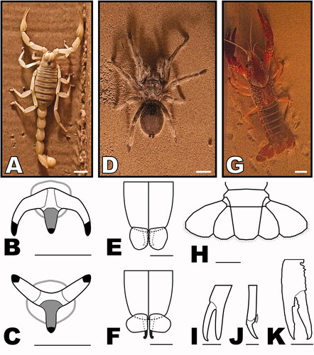
Figure 2. Drawings of some support structures used in spider, scorpion, and crayfish neoichnological experiments. Components were made out of wood or plexiglass, except for the aluminum pan holding the sand. (A) Drawing of the 15° angled wooden support structure made for dry/damp experiments (see C). (B) Drawing of the 15° angled plexiglass support structure for wet/subaqueous experiments (25° angled one not shown). (C) Drawing of the 25° angled wooden support structure, shown inside a dry aquarium.
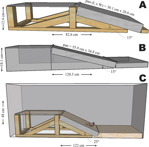
Figure 3. Examples of neoichnological experimental setups used to generate spider, scorpion, and crayfish trackways. (A) Dry aquarium (L: 122 cm; W: 30.5 cm; H: 48 cm) containing a wooden supporting platform with a 15° slope angle, suitable for dry or damp conditions; note the pieces of wood to contain and direct the animals. (B) The setup shown in (A) is at the top of the photo, showing dry sand and a shelter at the top to entice animals upwards; the bottom shows the larger tank (L: 122 cm; W: 38 cm; H: 40.5 cm) used for wet drying, wet saturated, or subaqueous experiments with the pan lying horizontal (0°) containing wet saturated sand with a plexiglass staging platform. (C) Setup for sloped, subaqueous scorpion experiments; cloudiness of water due to sand being reset multiple times after much trackway making (further experiments would have required changing the water or allowing clay particles to settle overnight).
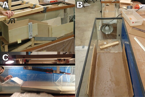
Table 1. Number of experimental runs, analyzed trackway segments (ATS), and symmetric ATS (Sym) per condition for scorpion, spider, and crayfish trackways.
Figure 4. Illustrated trackway terminology showing the measurements and some arthropod trackway characteristics examined in this study (q.v., ). The overall internal mark width (OIMW) refers to the total width of internal linear drag marks made by the crayfish tail fan, while the narrower internal linear marks could be made, for example, by a scorpion’s metasoma or only part of the crayfish’s tail fan.
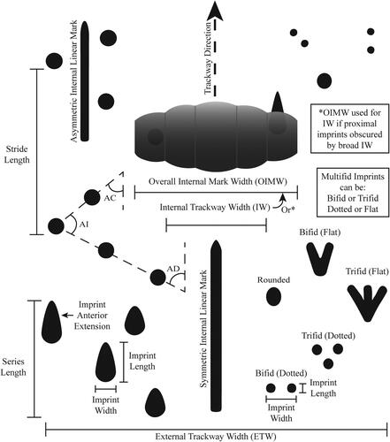
Table 2. List of important binary and ratio variables used in neoichnological experiments with scorpion, spider, and crayfish trackways, along with their abbreviations.
Table 3. Variables included or excluded (with reason given) in N-MDS visualizations for experimental tarantula, scorpion, and crayfish trackways.
Figure 5. Examples of experimental traces made by six Arizona desert hairy scorpions. The pictures are representative, but not necessarily comprehensive, in terms of the variability in morphology in each condition (water content + slope angle). Upslope is towards the top of the photos in the shallow and steep slope rows (not applicable to the first row which is flat without slope). Larger, annotated photographs of all the trackways analyzed in this study are available online via FigShare (Clendenon & Brand, Citation2024).
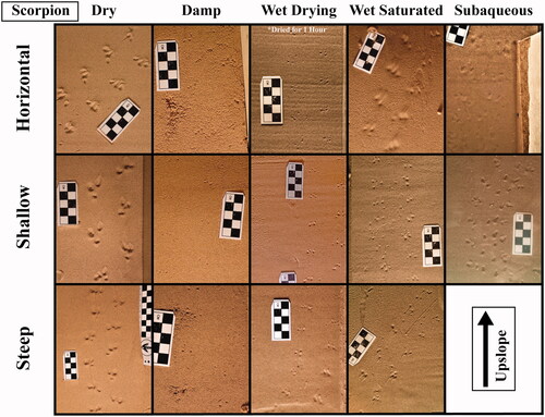
Figure 6. Examples of experimental traces made by two Chilean rose tarantulas. The pictures are representative, but not necessarily comprehensive, in terms of the variability in morphology in each condition (water content + slope angle). Upslope is towards the top of the photos in the shallow and steep slope rows (not applicable to the first row which is flat without slope). Larger, annotated photographs of all the trackways analyzed in this study are available online via FigShare (Clendenon & Brand, Citation2024).
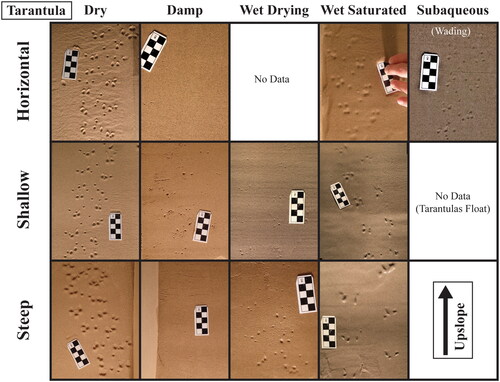
Figure 7. Examples of experimental traces made by four red swamp crayfish. The pictures are representative, but not necessarily comprehensive, in terms of the variability in morphology in each condition (water content + slope angle). Upslope is towards the top of the photos in the shallow and steep slope rows (not applicable to the first row which is flat without slope). Larger, annotated photographs of all the trackways analyzed in this study are available online via FigShare (Clendenon & Brand, Citation2024).
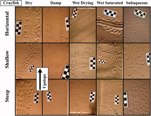
Figure 8. Clustered bar chart showing how often each imprint number category was found in the majority of series in all the analyzed trackway segments (ATS) for each type of invertebrate (species) producer. Percentages do not sum to 100% across number categories because the majority of series within an analyzed trackway segment may include multiple categories (e.g. approximately equal numbers of two- and three-imprint series), in which case each category was counted as present for that analyzed trackway segment. Minor series are excluded here.
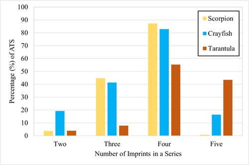
Figure 9. Clustered bar chart showing how often each series shape was found in the majority of series in all the analyzed trackway segments (ATS) for each type of invertebrate (species) producer. Percentages do not sum up to 100% across series shapes because the majority of series within an analyzed trackway segment may include multiple series shapes, in which case each category is counted as present for that analyzed trackway segment. Minor series are excluded here.
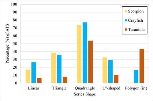
Table 4. External trackway width statistics (in mm ± SD) for each species and the five target conditions.
Figure 10. Binary variable trends for scorpion trackways split by five sand conditions (all slopes included in each of the five conditions, so variability due to slope is accounted for). Shown are the percentages of analyzed trackway segments (ATS) in a condition that are present and absent. Note that for “Symmetric Int. Lin. Marks” (= LM Asym), ATS without internal marks were not included in calculations of percent values. Tapering added to bars near 100% for visual clarity.
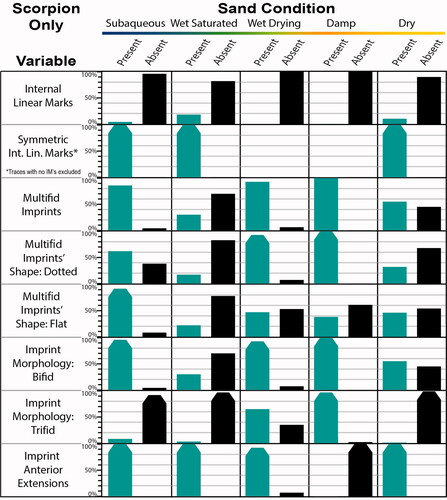
Figure 11. Experimental scorpion trackway trends for series shape and number of imprints per series, split by five sand conditions (all slopes included in each of the five conditions, so variability due to slope is accounted for). Shown are the percentages of analyzed trackway segments (ATS) in a condition that are present and absent. Tapering added to bars near 100% for visual clarity.
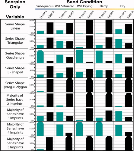
Figure 12. Range area charts showing ratio variable trends for scorpion trackways split by five sand conditions. The five conditions contain both flat and sloped trackways (as applicable), so variability due to slope is included in each condition. Shown, for each ratio in each condition, are the individual ratio values (%) for the analyzed trackway segments (ATS) having the maximum, median, and minimum ratio values in each condition. To better visualize how all the ratios vary together across conditions, the values are expressed as percentages (each value was divided by the maximum value amongst the experimental trackways for each ratio). Note that for OIMW/ETW, ATS without internal marks (i.e. OIMW/ETW = 0) were not included in calculations of percent values.
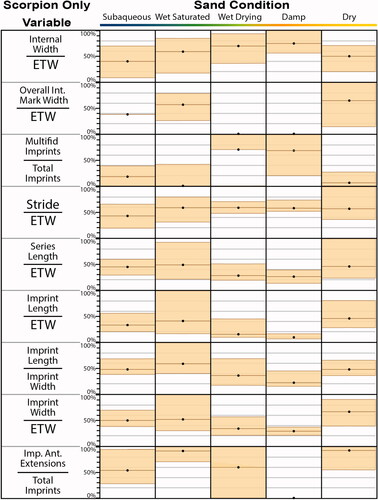
Figure 13. Binary variable trends for tarantula trackways split by five sand conditions (all slopes included in each of the five conditions, so variability due to slope is accounted for). Shown are the percentages of analyzed trackway segments (ATS) in a condition that are present and absent. Note that for “Symmetric Int. Lin. Marks” (= LM Asym), ATS without internal marks were not included in calculations of percent values. Tapering added to bars near 100% for visual clarity.
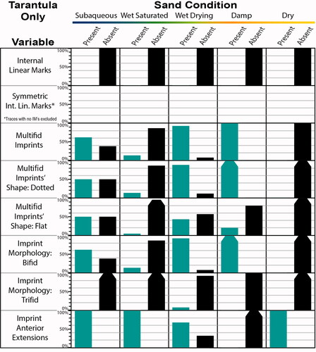
Figure 14. Experimental tarantula trackway trends for series shape and number of imprints per series, split by five sand conditions (all slopes included in each of the five conditions, so variability due to slope is accounted for). Shown are the percentages of analyzed trackway segments (ATS) in a condition that are present and absent. Tapering added to bars near 100% for visual clarity.
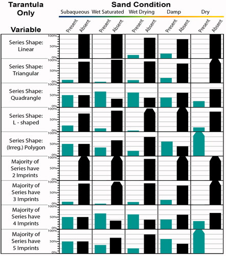
Figure 15. Range area charts showing ratio variable trends for tarantula trackways split by five sand conditions. For additional explanation, see caption.
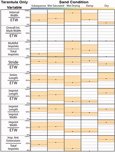
Figure 16. Binary variable trends for crayfish trackways split by five sand conditions (all slopes included in each of the five conditions, so variability due to slope is accounted for). Shown are the percentages of analyzed trackway segments (ATS) in a condition that are present and absent. Note, for “Symmetric Int. Lin. Marks” (= LM Asym), ATS without internal marks were not included in calculations of percent values. Tapering added to bars near 100% for visual clarity.
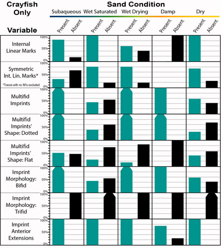
Figure 17. Experimental crayfish trackway trends for series shape and number of imprints per series, split by five sand conditions (all slopes included in each of the five conditions, so variability due to slope is accounted for). Shown are the percentages of analyzed trackway segments (ATS) in a condition that are present and absent. Tapering added to bars near 100% for visual clarity.
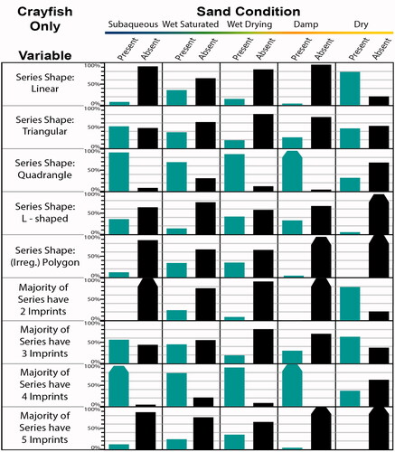
Figure 18. Range area charts showing ratio variable trends for crayfish trackways split by five sand conditions. For additional explanation, see caption.
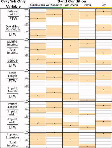
Figure 19. Non-metric multidimensional scaling (N-MDS) visualization for a random sample of scorpion trackways grouped by condition (N = 134; stress = 0.1604). For the variables used, see .
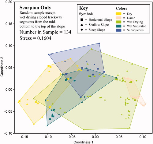
Figure 20. Non-metric multidimensional scaling (N-MDS) visualization for tarantula trackways grouped by condition (Overall N = 76; stress = 0.1199). For the variables used, see .
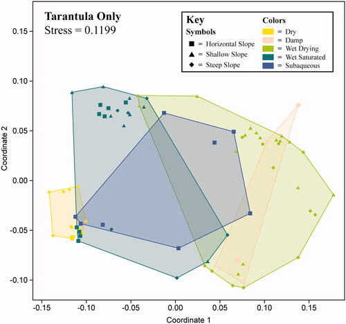
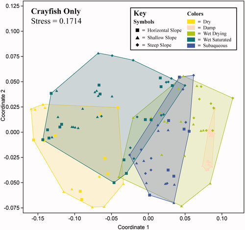
Figure 21. Non-metric multidimensional scaling (N-MDS) visualization for crayfish trackways grouped by five conditions (Overall N = 139; stress = 0.1714). For the variables used, see . Note how wet saturated (dark turquoise color) is in the left and center of the coordinate plane, and then moving to the bottom-right, transitions to wet drying (lighter green color) then damp (light peach color) as the sand conditions go from loose to stiff.
gich_a_2322937_sm3172.docx
Download MS Word (10.8 KB)Data availability statement
Annotated images of all experimental symmetric analyzed trackway segments, the primary data set with analyzed trackway segment parameters, and all Supplementary Materials are available online (DOI: 10.6084/m9.figshare.c.6778683) through FigShare (Clendenon & Brand, Citation2024).