Switching nonparametric regression models

Figures & data

Figure 1. Motorcycle data. Head acceleration in g (one g ≈ 9.8 m/s²) versus the time in milliseconds after impact.

Table 1.  Summary of the simulation studies.

Sim'n	Type of zis	zis parameters	s
1	iid	p1=0.7
		p2=0.3
2	Markov
		a12=0.3
		a21=0.4
3
		a12=0.1
		a21=0.2

Figure 2. Top row: Simulation 1 (iid z_is with p₁=0.7). Bottom row: Simulation 2 (Markov z_is with a₁₂=0.3 and a₂₁=0.4). Example of simulated data along with the initial and final estimates of f₁ and f₂ obtained using the Bayesian approach and the penalised log-likelihood approaches. The light-coloured dots correspond to z=2 and the dark-coloured dots to z=1. The solid lines correspond to the true functions f₁ and f₂, respectively. The dot-dashed lines are the initial estimates of f₁ and f₂ obtained using the function estimate method. The dashed lines are the final estimates of f₁ and f₂. See online version for colours.

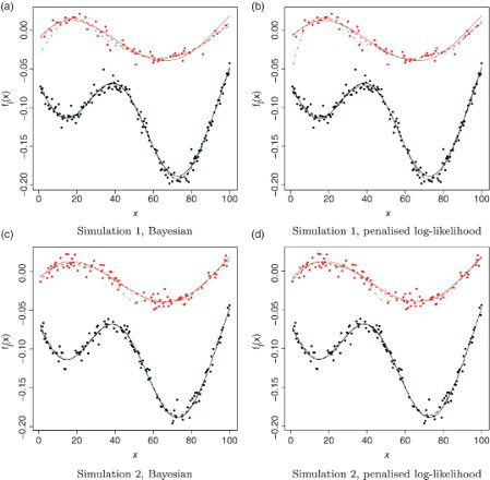
Figure 3. Simulation 3 (Markov z_is with a₁₂=0.1 and a₂₁=0.2). Top row: Example of simulated data along with the initial and final estimates of f₁ and f₂. The light-coloured dots correspond to z=2 and the dark-coloured dots to z=1. The solid lines correspond to the true functions f₁ and f₂, respectively. The dot-dashed lines are the initial estimates of f₁ and f₂ obtained using the residual-based method. The dashed lines are the final estimates of f₁ and f₂. Bottom row: Example of simulated datasets along with initial estimates (dot-dashed lines) that yield (c) good and (d) bad final function estimates (dashed lines) using the Bayesian approach. See online version for colours.

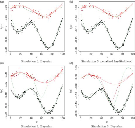
Figure 4. Top row: Simulation 1 (iid z_is with p₁=0.7). Bottom row: Simulation 3 (Markov z_is with a₁₂=0.1 and a₂₁=0.2). EMSE of the final estimates of f₁ and f₂ using the Bayesian (dashed lines) and the penalised log-likelihood (solid lines) approaches.

Table 2.  Number of simulated datasets with at least one value of pˆ(z_i=1|y_i)>0.2 when z_i=2.

Approach	Simulation 1	Simulation 2	Simulation 3
Bayes	0^a	0^a	4
Penalised log-likelihood	0^a	0^a	1

was never larger than 0.04 when the true z_i=2.

Table 3.  Number of simulated datasets with at least one value of pˆ(z_i=2|y_i)>0.2 when z_i=1.

Approach	Simulation 1	Simulation 2	Simulation 3
Bayes	3	3	14
Penalised log-likelihood	2	1	13

Table 4.  Estimates of σ² (true value=5×10⁻⁵).

Simulation	Approach	(SD)
1	Bayesian	4.984 (0.491)
	PL^b	4.912 (0.498)
2	Bayesian	4.982 (0.556)
	PL	4.916 (0.579)
3	Bayesian	4.935 (0.517)
	PL	4.880 (0.519)

^aSD, standard deviation.

^bPL, penalised log-likelihood.

Table 5.  Estimates of the parameters of the z process.

					Empirical coverage
Sim'n	z Parameters	Approach	Mean (SD^a)	Mean of SEs	90%	95%
1	p1=0.7	Bayesian	0.699 (0.032)	0.032	90.7%	95.7%
		PL^b	0.699 (0.032)	0.032	90.7%	95.7%
2	a12=0.3	Bayesian	0.300 (0.043)	0.043	90.0%	94.3%
		PL	0.300 (0.043)	0.043	90.0%	94.3%
	a21=0.4	Bayesian	0.399 (0.053)	0.053	90.3%	95.7%
		PL	0.399 (0.053)	0.053	90.3%	95.7%
3	a12=0.1	Bayesian	0.105 (0.025)	0.027	93.0%	97.3%
		PL	0.105 (0.024)	0.027	93.3%	97.3%
	a21=0.2	Bayesian	0.208 (0.052)	0.050	91.7%	92.7%
		PL	0.208 (0.052)	0.050	91.7%	92.7%

^aSD, standard deviation.

^bPL, penalised log-likelihood.

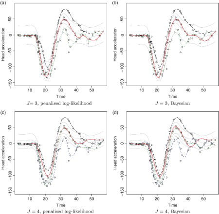
Figure 5. Motorcycle data. Top row: final function estimates obtained for J=3 using (a) the penalised log-likelihood approach and (b) the Bayesian approach. Bottom row: final function estimates obtained for J=4 using (c) the penalised log-likelihood approach and (d) the Bayesian approach. The thin light-coloured lines correspond to the initial function estimates, which are constant shifts of a smoothing spline fit to all the data. See online version for colours.

Table 6.  Results for J=3 with corresponding fitted curves in Figure 5(a) and 5(b).

Approach	Curve		pˆj (s.e.)	λj
Penalised	Black (long-dashed)	43.054	0.269 (0.047)	0.893
Log-likelihood	Red (solid)	14.227	0.395 (0.053)	0.890
(Figure 5(a))	Green (dot-dashed)	171.048	0.337 (0.053)	0.167
Bayesian	Black (long-dashed)	50.134	0.272 (0.047)	3.901
(Figure 5(b))	Red (solid)	8.593	0.361 (0.050)	5.005
	Green (dot-dashed)	184.478	0.367 (0.052)	2.512

Table 7.  Results for J=4 with corresponding fitted curves in Figure 5(c) and 5(d).

Approach	Curve		pˆj (s.e.)	λj
Penalised	Black (long-dashed)	50.348	0.211 (0.042)	1.591
Log-likelihood	Red (solid)	7.623	0.232 (0.050)	1.213
(Figure 5(c))	Green (dot-dashed)	7.245	0.244 (0.051)	0.825
	Blue (dashed)	135.968	0.313 (0.049)	0.545
Bayesian	Black (long-dashed)	48.376	0.223 (0.043)	3.782
(Figure 5(d))	Red (solid)	5.473	0.221 (0.045)	4.805
	Green (dot-dashed)	1.106	0.198 (0.042)	5.377
	Blue (dashed)	145.440	0.358 (0.048)	3.355