Do Areas Affected by Flood Disasters Attract Lower-Income and Less Creditworthy Homeowners?

Figures & data

Figure 1. Map of counties selected for the study.

Note. This map shows the counties selected for our study. These are the counties that experienced a major flood disaster but were not affected by a similar disaster in the preceding three years and the following two years. Darker shades represent more recent disaster declarations, and lighter shades represent older disasters. Only the most recent disaster is included for counties that appear more than once in the sample.

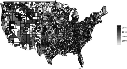
Table 1. Summary statistics: Mortgage applications sample.

Panel A: Applications
	Mean	St. Dev.	Pctl(25)	Median	Pctl(75)	N
Applicant’s income ($ 000)	95	122	48	72	110	56,357,839
Loan amount ($ 000)	202	245	98	158	256	62,514,466
White	0.65	0.48	0.00	1.00	1.00	62,514,466
New purchase	0.45	0.50	0.00	0.00	1.00	62,514,466
Owner-occupied	0.95	0.22	1.00	1.00	1.00	62,514,466
Originated	0.46	0.50	0.00	0.00	1.00	62,514,466
Panel B: Originated Mortgages
	Mean	St. Dev.	Pctl(25)	Median	Pctl(75)	N
Applicant’s income ($ 000)	101	111	51	77	118	28,507,796
Loan amount ($ 000)	209	192	100	164	265	28,586,337
White	0.77	0.42	1.00	1.00	1.00	28,586,337
New purchase	0.50	0.50	0.00	1.00	1.00	28,586,337
Owner-occupied	0.94	0.24	1.00	1.00	1.00	28,586,337
Securitized	0.39	0.49	0.00	0.00	1.00	28,586,337
Panel C: Originated Mortgages - Before Vs. After Flood Disaster
	Before Disaster			After Disaster
	Mean	St. Dev.	N	Mean	St. Dev.	N
Applicant’s income	103.3304	109.3295	18,991,599	96.5785	113.0538	9,516,197
Loan amount	220.8786	196.1735	19,036,398	184.7429	180.3069	9,549,939
White	0.7644	0.4243	19,036,398	0.7877	0.4090	9,549,939
New purchase	0.4938	0.5000	19,036,398	0.5182	0.4997	9,549,939
Owner-occupied	0.9417	0.2343	19,036,398	0.9307	0.2540	9,549,939
Securitized	0.3949	0.4888	19,036,398	0.3900	0.4877	9,549,939

Note. This table shows sample means and standard deviations of key variables of the mortgage applications sample. This sample consists of mortgage applications three years before, during, and two years after the respective disaster declaration in each county. Sample excludes multi-unit multi-family homes and home equity loans. Mortgage applications data is from the year 2004. Sample in Panel A includes all the mortgage applications and sample in Panel B is restricted to only successful mortgage applications. In Panel C, we further divide the sample into mortgages originated before and after the disaster.

Table 2. Summary statistics: Mortgage performance sample.

Panel A. Sample Means and Standard Deviations
Statistic	Mean	St. Dev.	Pctl(25)	Median	Pctl(75)	N
Disaster year	2004.57	1.58	2004	2005	2006	696,799
FICO Score	662	70	610	659	715	676,392
Interest rate	7.39	1.97	6.25	7.25	8.50	696,617
Loan-to-value	87	13	80	90	100	679,851
Loan amount	180,384	188,887	83,000	125,900	205,600	696,798
Fixed rate loan	0.42	0.49	0.00	0.00	1.00	696,799
Full documentation	0.47	0.50	0.00	0.00	1.00	696,799
Owner-occupied	0.87	0.34	1.00	1.00	1.00	696,799
New purchase	0.73	0.45	0.00	1.00	1.00	696,799
Panel B. Performance Before Vs. After Flood Disaster
	Before Disaster			After Disaster
	Mean	St. Dev.	N	Mean	St. Dev.	N
FICO Score	663.78	70.40	157,944	661.56	69.73	342,269
Interest rate	7.25	1.91	164,223	7.56	2.01	349,869
Loan-to-value	86.30	13.24	160,227	87.60	12.91	342,048
Loan amount	195,466.00	191,918.00	164,258	177,220.30	170,396.50	349,961
Fixed rate loan	0.40	0.49	164,258	0.44	0.50	349,962
Full documentation	0.44	0.50	164,258	0.49	0.50	349,962
Owner-occupied	0.88	0.32	164,258	0.86	0.35	349,962
New purchase	0.69	0.46	164,258	0.74	0.44	349,962
Debt-to-income	15.54	19.85	63,351	25.77	19.88	125,971

Note. Panel A of this table shows sample means and standard deviations of key variables of the mortgage performance sample. This sample consists of mortgages originated three years before, during, and two years after the respective disaster declaration in each county. Sample excludes multi-unit multi-family homes and home equity loans. We also restrict the sample to mortgages with a 30-year term. Panel B divides the sample into mortgages originated before and after the disaster declaration.

Figure 2. Impact of flood disasters on house prices and market activity.

$$Y_{\mathit{igty}}={\beta }_t\times t+\mathit{\delta }{\mathit{X}}_i+{\mu }_g+{\mu }_y+c_{\mathit{igty}}$$

Note. This figure presents the estimation results of regressions aimed at understanding the changes to house prices and the number of homes sold in a ZIP code after a flood disaster. The y -axis plots the estimated β_t and the corresponding confidence intervals of the following specification. t represents dummy variables that indicate the number of years since the flood disaster in ZIP code g. The dependent variables in Panel A and Panel B are log(house price) and log(number of homes sold) respectively. μ_g and μ_y are ZIP code and calendar year fixed effects, respectively.

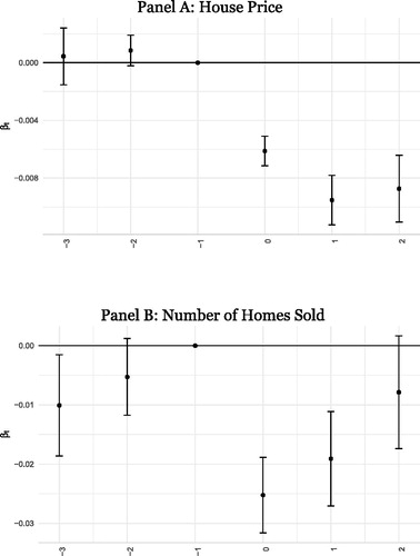
Figure 3. Mortgage applicants’ income after flood disasters (staggered DiD).

$$Y_{\mathit{igty}}={\beta }_t\times t+\mathit{\delta }{\mathit{X}}_i+{\mu }_g+{\mu }_y+c_{\mathit{igty}}$$

Note. This figure presents the estimation results of regressions aimed at understanding the changes to mortgage applicants’ income after a flood disaster. The y -axis plots the estimated β_t and the corresponding confidence intervals of the following specification. t represents dummy variables that indicate the number of years since the flood disaster in census tract g. The dependent variables is log(mortgage applicant’s income) and μ_g and μ_y are census tract and calendar year fixed effects respectively. The sample consists of successful mortgage applications to purchase owner-occupied homes.

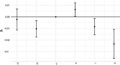
Table 3. Mortgage applicants’ income after flood disasters (staggered DiD).

	(1)	(2)
Post	−0.015***	−0.016***
	(0.001)	(0.001)
White		0.005***
		(0.001)
log(Loan amount)		0.527***
		(0.004)
Census tract	✓	✓
Year	✓	✓
Observations	6,224,962	6,224,962
Adjusted R^2	0.293	0.430

Note. This table reports the results of the regressions that examine the difference in the mortgage applicants’ income before and after the flood disaster. The dummy variable post takes the value of one if the mortgage was originated after the flood disaster. The dependent variables is log(mortgage applicant’s income). Sample consists of successful mortgage applications to finance owner-occupied new home purchases. Standard errors are clustered at census tract level and reported in parentheses below coefficient estimates. We use *,**, and *** to denote statistical significance at the 10%, 5%, and 1% levels, respectively.

Figure 4. Changes in new home purchasers’ income relative to the control groups.

$$Y_{\mathit{igty}}={\beta }_t\times t\times \mathit{treate}{d}_{\mathit{igty}}+\mathit{\delta }{\mathit{X}}_i+{\mu }_{gy}+c_{\mathit{igty}}$$

Note. This figure presents estimation results of regressions aimed at understanding the changes to the income of mortgage applicants who are purchasing new homes relative to mortgage applicants who are just refinancing and relative to mortgage applicants who are purchasing non-owner-occupied homes. The y -axis plots the estimated β_t and the corresponding confidence intervals of the following specification. t represents dummy variables that indicate the number of years since the flood disaster in census tract g.

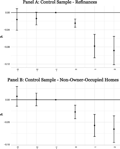
Table 4. Mortgage applicants’ income after flood disasters (generalized DiD).

	(1)	(2)
Control Sample	Refinance	Non-owner-occupied
Treated × Post	−0.070*** (0.001)	−0.058*** (0.003)
Treated	−0.073*** (0.002)	−0.645*** (0.002)
Post	0.025*** (0.002)	0.053*** (0.001)
White	0.008*** (0.001)	0.006*** (0.001)
log(Loan amount)	0.503*** (0.003)	0.508*** (0.004)
Census tract × Year	✓	✓
Observations	6,224,962	6,224,962
Adjusted R^2	0.293	0.430

Note. This table reports the results of the regressions that examine the difference in the mortgage applicants’ income before and after the flood disaster compared to two control groups. Column (1) uses mortgages that refinanced existing mortgages as the control sample, and Column (2) uses mortgages that financed the purchase of non-owner-occupied homes as the control sample. The dummy variables post and treated takes the value of one if the mortgage was originated after the flood disaster and financed the purchase of an owner-occupied home purchase respectively. The dependent variables is log(mortgage applicant’s income). Standard errors are clustered at census tract level and reported in parentheses below coefficient estimates. We use *,**, and *** to denote statistical significance at the 10%, 5%, and 1% levels, respectively.

Table 5. Mortgage applicants’ income after repeated flood disasters.

Note. This table reports the results of the regressions that compares the difference in the mortgage applicants’ income before and after the repeated flood disasters. Column (1) compares the changes in income of mortgage applicants after the subsequent disasters with the same after the first disaster that affected the same area during the sample period. Columns (2) and (3) do the same analysis using refinance mortgage applications, and non-owner-occupied mortgage applications as control samples, respectively. The dummy variables Post, Treated, and Repeated take the value of one if the mortgage was originated after the flood disaster, financed the purchase of an owner-occupied home purchase, and the disaster is not the first disaster affecting the same area in the sample respectively. The dependent variables is log(mortgage applicant’s income). Standard errors are clustered at census tract level and reported in parentheses below coefficient estimates. We use *, **, and *** to denote statistical significance at the 10%, 5%, and 1% levels, respectively.

Figure 5. Mortgage delinquency rates (staggered DiD).

$$Y_{\mathit{igty}}={\beta }_t\times t+\mathit{\delta }{\mathit{X}}_i+{\mu }_g+{\mu }_y+c_{\mathit{igty}}$$

Note. This figure presents the estimation results of regressions aimed at understanding the difference in the likelihood of mortgage borrowers to become seriously delinquent, depending on whether the mortgage was originated before or after the disaster. The y -axis plots the estimated β_t and the corresponding confidence intervals of the following specification. t represents dummy variables that indicate the number of quarters since the flood disaster in ZIP code g. The dependent variable is a dummy variable that indicates whether the mortgage became 150 days or more delinquent at some point after origination. μ_g and μ_y are ZIP code and calendar quarter fixed effects, respectively.

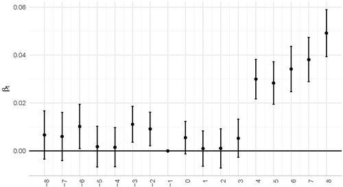
Table 6. Mortgage delinquency rates (staggered DiD).

	(1)	(2)
Post	0.085***	0.084***
	(0.004)	(0.004)
log(FICO Score)		−0.875***
		(0.011)
log(Interest rate)		−0.067***
		(0.003)
log(Loan-to-value)		0.162***
		(0.005)
log(Loan amount)		−0.008***
		(0.001)
Full documentation		0.014***
		(0.001)
Fixed rate loan		0.092***
		(0.002)
Zip code	✓	✓
Year	✓	✓
Observations	468,793	444,457
Adjusted R^2	0.061	0.103

Note. This table reports the results of the regressions that examine the difference in the likelihood of mortgage borrowers to become seriously delinquent, depending on whether the mortgage was originated before or after the disaster. The dummy variable post takes the value of one if the mortgage was originated after the flood disaster. The dependent variable is a dummy variable that indicates whether the mortgage became 150 days or more delinquent at some point after origination. Standard errors are clustered at ZIP code level and reported in parentheses below coefficient estimates. We use *,**, and *** to denote statistical significance at the 10%, 5%, and 1% levels, respectively.

Figure 6. Differences in delinquency rates compared to control groups.

$$Y_{\mathit{igty}}={\beta }_t\times t\times \mathit{treate}{d}_{\mathit{igty}}+\mathit{\delta }{\mathit{X}}_i+{\mu }_{gy}+c_{\mathit{igty}}$$

Note. This figure presents estimation results of regressions aimed at understanding the differences in the probability of default of mortgages that finance new purchases of owner-occupied homes relative to mortgages that refinance existing mortgages or mortgages that finance the purchases of non-owner-occupied homes. The y -axis plots the estimated β_t and the corresponding confidence intervals of the following specification. t represents dummy variables that indicate the number of quarters since the flood disaster in ZIP code g. The dependent variable is a dummy variable that indicates whether the mortgage became 150 days or more delinquent at some point after origination. μ_gy are census tract calendar year fixed effects. Controls samples in Panel A and Panel B refinance mortgages and non-owner-occupied home purchase mortgages, respectively.

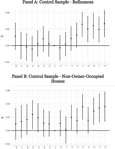
Table 7. Mortgage delinquency rates (generalized DiD).

	(1)	(2)
Control Sample	Refinance	Non-owner-occupied
Treated × Post	0.012*** (0.003)	0.006* (0.004)
Treated	0.023*** (0.003)	0.032*** (0.003)
Post	−0.012** (0.005)	−0.011* (0.006)
log(Interest rate)	−0.087*** (0.003)	−0.089*** (0.003)
log(FICO Score)	−0.816*** (0.011)	−0.855*** (0.013)
log(Loan-to-value)	0.168*** (0.005)	0.147*** (0.005)
log(Loan amount)	−0.020*** (0.001)	−0.025*** (0.002)
Full documentation	0.002 (0.001)	0.006*** (0.002)
Fixed rate loan	0.072*** (0.002)	0.072*** (0.002)
Zip code × quarter	✓	✓
Observations	629,068	521,449
Adjusted R^2	0.122	0.128

Note. This table reports the results of the regressions that examine the difference in the likelihood of owner-occupied mortgage borrowers to become seriously delinquent compared to two control samples. Column (1) uses mortgages that refinanced existing mortgages as the control sample, and Column (2) uses mortgages that financed the purchase of non-owner-occupied homes as the control sample. The dummy variables post and treated takes the value of one if the mortgage was originated after the flood disaster and financed the purchase of an owner-occupied home purchase respectively. The dependent variable is a dummy variable that indicates whether the mortgage became 150 days or more delinquent at some point after origination. Standard errors are clustered at ZIP code level and reported in parentheses below coefficient estimates. We use *,**, and *** to denote statistical significance at the 10%, 5%, and 1% levels, respectively..

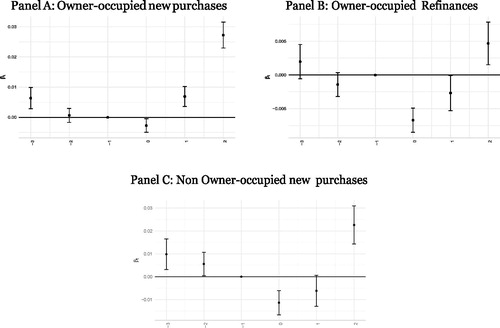
Figure 7. Mortgage interest rates (staggered DiD).

$$Y_{\mathit{igty}}={\beta }_t\times t+\mathit{\delta }{\mathit{X}}_i+{\mu }_g+{\mu }_y+c_{\mathit{igty}}$$

Note. This figure presents the estimation results of regressions aimed at understanding the changes to interest rates charged by mortgage lenders after a flood disaster. The y -axis plots the estimated β_t and the corresponding confidence intervals of the following specification. t represents dummy variables that indicate the number of quarters since the flood disaster in ZIP code g. The dependent variables is log(interest rate) and μ_g and μ_y are ZIP code and calendar quarter fixed effects respectively. Samples in Panels A, B, and C consist of mortgages used to finance new purchases of owner-occupied homes, refinance existing mortgages backed by owner-occupied homes, and new purchases of non-owner-occupied homes, respectively.

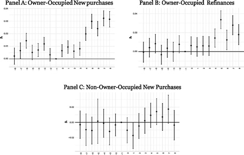
Figure 8. Likelihood to securitize (staggered DiD).

$$Y_{\mathit{igty}}={\beta }_t\times t+\mathit{\delta }{\mathit{X}}_i+{\mu }_g+{\mu }_y+c_{\mathit{igty}}$$

Note. This figure presents the estimation results of regressions aimed at understanding the changes to the probability of securitizing mortgages originated after a flood disaster. The y -axis plots the estimated β_t and the corresponding confidence intervals of the following specification. t represents dummy variables that indicate the number of years since the flood disaster in census tract g. The dependent variable is a dummy variable that indicates whether a particular mortgage i was securitized and μ_g and μ_y are census tract and calendar year fixed effects, respectively. Samples in Panels A, B, and C consist of mortgages used to finance new purchases of owner-occupied homes, refinance existing mortgages backed by owner-occupied homes, and new purchases of non-owner-occupied homes respectively.