1,635
Views
6
CrossRef citations to date
0
Altmetric
Original Articles

Bayesian Evidence Accumulation in Experimental Mathematics: A Case Study of Four Irrational Numbers

&

Figures & data

Figure 1. Sequential Bayes factors in favor of equal occurrence probabilities based on the first 100 million digits of π. The results in the top part of the panel correspond to an uninformative D(a = 1) prior for the alternative hypothesis; the results in the lower part of the panel correspond to the use of an informative D(a = 50) prior. The red lines indicate the maximum possible evidence for , and the gray areas indicate where 95% of the Bayes factors would fall if were true. After 100 million digits, the final Bayes factor under a D(a = 1) prior is BF01 = 1.86 × 1030 (log BF01 = 69.70); under a D(a = 50) prior, the final Bayes factor equals BF01 = 1.92 × 10²² (log BF01 = 51.31). Figure available at http://tinyurl.com/zelm4o4 under CC license https://creativecommons.org/licenses/by/2.0/.
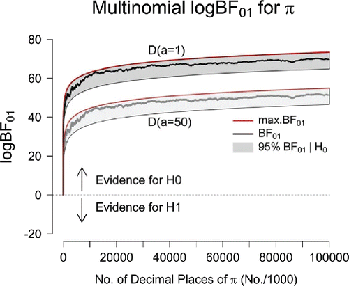
Figure 1. Sequential Bayes factors in favor of equal occurrence probabilities based on the first 100 million digits of π. The results in the top part of the panel correspond to an uninformative D(a = 1) prior for the alternative hypothesis; the results in the lower part of the panel correspond to the use of an informative D(a = 50) prior. The red lines indicate the maximum possible evidence for , and the gray areas indicate where 95% of the Bayes factors would fall if were true. After 100 million digits, the final Bayes factor under a D(a = 1) prior is BF01 = 1.86 × 1030 (log BF01 = 69.70); under a D(a = 50) prior, the final Bayes factor equals BF01 = 1.92 × 10²² (log BF01 = 51.31). Figure available at http://tinyurl.com/zelm4o4 under CC license https://creativecommons.org/licenses/by/2.0/.

Figure 2. Sequential Bayes factors in favor of equal occurrence probabilities based on the first 100 million digits of e. The results in the top part of the panel correspond to an uninformative D(a = 1) prior for the alternative hypothesis; the results in the lower part of the panel correspond to the use of an informative D(a = 50) prior. The red lines indicate the maximum possible evidence for , and the gray areas indicate where 95% of the Bayes factors would fall if were true. After 100 million digits, the final Bayes factor under a D(a = 1) prior is BF01 = 2.61 × 1030 (log BF01 = 70.04); under a D(a = 50) prior, the final Bayes factor equals BF01 = 2.69 × 10²² (log BF01 = 51.65). Figure available at http://tinyurl.com/h3wenqo under CC license https://creativecommons.org/licenses/by/2.0/.
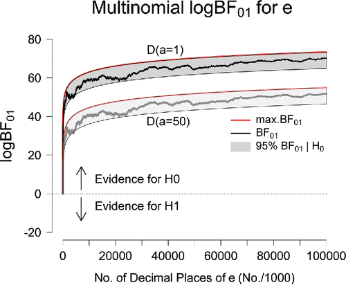
Figure 2. Sequential Bayes factors in favor of equal occurrence probabilities based on the first 100 million digits of e. The results in the top part of the panel correspond to an uninformative D(a = 1) prior for the alternative hypothesis; the results in the lower part of the panel correspond to the use of an informative D(a = 50) prior. The red lines indicate the maximum possible evidence for , and the gray areas indicate where 95% of the Bayes factors would fall if were true. After 100 million digits, the final Bayes factor under a D(a = 1) prior is BF01 = 2.61 × 1030 (log BF01 = 70.04); under a D(a = 50) prior, the final Bayes factor equals BF01 = 2.69 × 10²² (log BF01 = 51.65). Figure available at http://tinyurl.com/h3wenqo under CC license https://creativecommons.org/licenses/by/2.0/.

Figure 3. Sequential Bayes factors in favor of equal occurrence probabilities based on the first 100 million digits of . The results in the top part of the panel correspond to an uninformative D(a = 1) prior for the alternative hypothesis; the results in the lower part of the panel correspond to the use of an informative D(a = 50) prior. The red lines indicate the maximum possible evidence for , and the gray areas indicate where 95% of the Bayes factors would fall if were true. After 100 million digits, the final Bayes factor under a D(a = 1) prior is BF01 = 7.29 × 1030 (log BF01 = 71.06); under a D(a = 50) prior, the final Bayes factor equals BF01 = 7.52 × 10²² (log BF01 = 52.67). Figure available at http://tinyurl.com/jgwu523 under CC license https://creativecommons.org/licenses/by/2.0/.
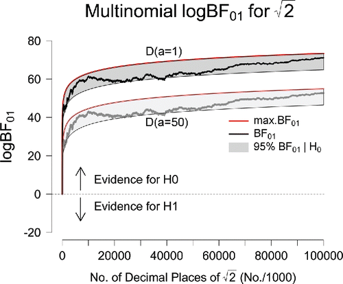
Figure 3. Sequential Bayes factors in favor of equal occurrence probabilities based on the first 100 million digits of . The results in the top part of the panel correspond to an uninformative D(a = 1) prior for the alternative hypothesis; the results in the lower part of the panel correspond to the use of an informative D(a = 50) prior. The red lines indicate the maximum possible evidence for , and the gray areas indicate where 95% of the Bayes factors would fall if were true. After 100 million digits, the final Bayes factor under a D(a = 1) prior is BF01 = 7.29 × 1030 (log BF01 = 71.06); under a D(a = 50) prior, the final Bayes factor equals BF01 = 7.52 × 10²² (log BF01 = 52.67). Figure available at http://tinyurl.com/jgwu523 under CC license https://creativecommons.org/licenses/by/2.0/.

Figure 4. Sequential Bayes factors in favor of equal occurrence probabilities based on the first 100 million digits of ln 2. The results in the top part of the panel correspond to an uninformative D(a = 1) prior for the alternative hypothesis; the results in the lower part of the panel correspond to the use of an informative D(a = 50) prior. The red lines indicate the maximum possible evidence for , and the gray areas indicate where 95% of the Bayes factors would fall if were true. After 100 million digits, the final Bayes factor under a D(a = 1) prior is BF01 = 7.58 × 1029 (log BF01 = 68.80); under a D(a = 50) prior, the final Bayes factor equals BF01 = 7.81 × 10²¹ (log BF01 = 50.41). Figure available at http://tinyurl.com/jqdyd3w under CC license https://creativecommons.org/licenses/by/2.0/.
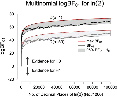
Figure 4. Sequential Bayes factors in favor of equal occurrence probabilities based on the first 100 million digits of ln 2. The results in the top part of the panel correspond to an uninformative D(a = 1) prior for the alternative hypothesis; the results in the lower part of the panel correspond to the use of an informative D(a = 50) prior. The red lines indicate the maximum possible evidence for , and the gray areas indicate where 95% of the Bayes factors would fall if were true. After 100 million digits, the final Bayes factor under a D(a = 1) prior is BF01 = 7.58 × 1029 (log BF01 = 68.80); under a D(a = 50) prior, the final Bayes factor equals BF01 = 7.81 × 10²¹ (log BF01 = 50.41). Figure available at http://tinyurl.com/jqdyd3w under CC license https://creativecommons.org/licenses/by/2.0/.

Figure 5. Sequential Bayes factors in favor of equal occurrence probabilities based on the first 100 million digits of π, e, , and ln 2. The results correspond to the use of a two-component mixture prior of a D(a1 = 5) and D(a2 = 1/5) Dirichlet distribution where the mixing weight was equal to w = 0.5. The red lines indicate the maximum possible evidence for , and the gray areas indicate where 95% of the Bayes factors would fall if were true. Figure available at http://tinyurl.com/hw4gmlr under CC license https://creativecommons.org/licenses/by/2.0/.
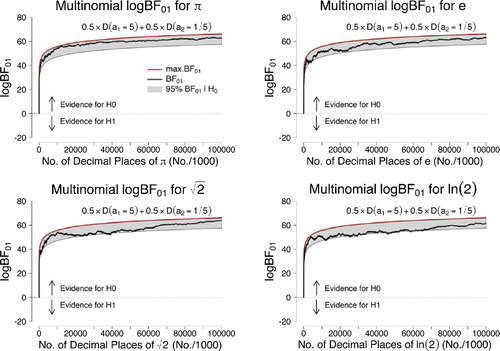
Figure 5. Sequential Bayes factors in favor of equal occurrence probabilities based on the first 100 million digits of π, e, , and ln 2. The results correspond to the use of a two-component mixture prior of a D(a1 = 5) and D(a2 = 1/5) Dirichlet distribution where the mixing weight was equal to w = 0.5. The red lines indicate the maximum possible evidence for , and the gray areas indicate where 95% of the Bayes factors would fall if were true. Figure available at http://tinyurl.com/hw4gmlr under CC license https://creativecommons.org/licenses/by/2.0/.

Figure 6. Sequential Bayes factors in favor of equal occurrence probabilities based on the first 100 million digits of π, e, , and ln 2. The results in the upper panel correspond to the use of an uninformative D(a = 1) prior for the alternative hypothesis; the results in the middle panel correspond to the use of an informative D(a = 50) prior; the results in the lower panel correspond to the use of a two-component mixture prior of a D(a1 = 5) and D(a2 = 1/5) Dirichlet distribution where the mixing weight was equal to w = 0.5. Figure available at http://tinyurl.com/hhut8dp under CC license https://creativecommons.org/licenses/by/2.0/.
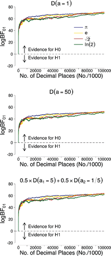
Figure 6. Sequential Bayes factors in favor of equal occurrence probabilities based on the first 100 million digits of π, e, , and ln 2. The results in the upper panel correspond to the use of an uninformative D(a = 1) prior for the alternative hypothesis; the results in the middle panel correspond to the use of an informative D(a = 50) prior; the results in the lower panel correspond to the use of a two-component mixture prior of a D(a1 = 5) and D(a2 = 1/5) Dirichlet distribution where the mixing weight was equal to w = 0.5. Figure available at http://tinyurl.com/hhut8dp under CC license https://creativecommons.org/licenses/by/2.0/.

Figure 7. Sequential Bayes factors in favor of equal occurrence probabilities for 1,000 simulated data sets of 1 million digits each. In every data set, one digit was given an occurrence probability of.11 whereas each of the other digits occurred with probability .89/9. The evidential trajectories indicate increasingly strong evidence against the general law. Figure available at http://tinyurl.com/j4qk2ht under CC license https://creativecommons.org/licenses/by/2.0/.
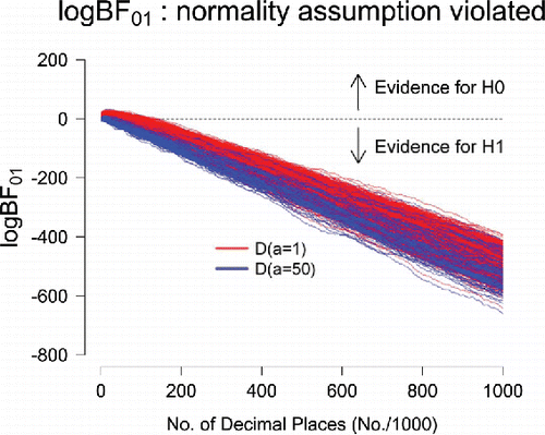
Figure 7. Sequential Bayes factors in favor of equal occurrence probabilities for 1,000 simulated data sets of 1 million digits each. In every data set, one digit was given an occurrence probability of.11 whereas each of the other digits occurred with probability .89/9. The evidential trajectories indicate increasingly strong evidence against the general law. Figure available at http://tinyurl.com/j4qk2ht under CC license https://creativecommons.org/licenses/by/2.0/.
Supplemental material

UEXM_A_1256006_supplemental_material.docx

Download MS Word (11.2 KB)