Adventures in Supersingularland

Figures & data

Fig. 1 The graph ${\mathcal{G}}_2({\mathbb{F}}_p)$ for p = 431 (case 3.a of Theorem 3.5). The vertices are labeled by j-invariants of each curve. Each component is a volcano, with an inner ring of surface curves and the outer vertices all being curves on the floor. The class number of $\mathbb{Q}\left(\sqrt{-431}\right)$ is $3·7=21$ and the orders of the two primes above 2 are 7.

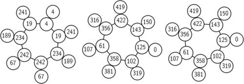
Fig. 2 Stacking, folding and attaching by an edge for p = 431 and $\mathcal{l}=2$. The leftmost component of ${\mathcal{G}}_2({\mathbb{F}}_p)$ folds, the other two components stack, and the vertices 189 and 150 get attached by a double edge.

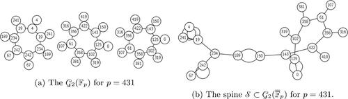
Fig. 3 Attachment along a j-invariant for p = 83 and $\mathcal{l}=3$. The two connected components of ${\mathcal{G}}_3({\mathbb{F}}_p)$ are attached along the j-invariant $68=1728\text{mod}83$. There are two outgoing double edges from j = 1728 but because of the extra automorphisms, these edges are identified in the undirected graph.

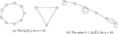
Fig. 4 Attachment by an edge that does not attach two distinct components. This component folds and the vertices with j-invariants 68 and 107 are joined by a double edge.

Table

Residue class of p	Endomorphism rings	Shape of ${\mathcal{G}}_2({\mathbb{F}}_p)$
$p\equiv 1\text{mod}4$	$\mathbb{Z}[\sqrt{-p}]$	Each connected component is two vertices connected by one edge, corresponding to a horizontal isogeny (see Figure 6(a)).
$p\equiv 3\text{mod}8$	$\mathbb{Z}[\sqrt{-p}],\mathbb{Z}\left[\frac{1+\sqrt{-p}}{2}\right]$	Each connected component is “claw”: one vertex on the surface connected to three vertices on the floor by vertical isogenies (see Figure 6(b).)
$p\equiv 7\text{mod}8$	$\mathbb{Z}[\sqrt{-p}],\mathbb{Z}\left[\frac{1+\sqrt{-p}}{2}\right]$	Each connected component is a 2-level “volcano” with surface a cycle of size $\ge 1$. From any vertex on the surface there is exactly one vertical isogeny. There are no horizontal isogenies on the floor (see Figure 1.)

Fig. 5 The graph ${\mathcal{G}}_3({\mathbb{F}}_p)$ for p = 179. We see that the neighbors of vertices with j-invariant 0 both have j-invariant $-12288000\text{mod}179=171$.

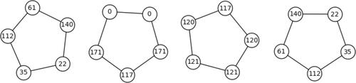
Fig. 6 Possible shapes for ${\mathcal{G}}_2({\mathbb{F}}_p)$ for $p\equiv 1\text{mod}4$ (left) and $p\equiv 3\text{mod}8$.

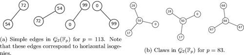
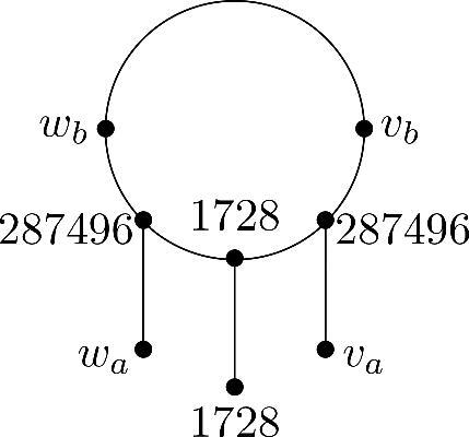
Fig. 7 The double edge from j to $\mathbf{j}\prime$.

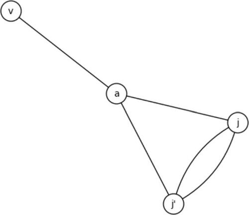
Fig. 8 Comparing average distances between random vertices in ${\mathcal{G}}_2({\overline{\mathbb{F}}}_p)$ and between connected components of $\mathcal{S}\subset {\mathcal{G}}_2({\overline{\mathbb{F}}}_p)$. On the horizontal axis, we have primes $p\equiv 1\text{mod}4$. The height of each point represents (avg. distance between ${\mathbb{F}}_p$-components) - (avg. distance between 100 random points of ${\mathcal{G}}_2({\overline{\mathbb{F}}}_p)$).

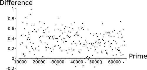
Table 1 Size and shape of the spine, depending on primes modulo 8, the integer n denotes the order of any prime above 2 in $\text{cl}({\mathcal{O}}_K)$.

prime mod 8	shape of ${\mathcal{G}}_2({\mathbb{F}}_p)$	$\#\mathcal{S}$	$\approx \#(\mathcal{S}$-Components)
$1\text{mod}4$	edges	$\frac{1}{2}h(-4p)$	$\frac{1}{4}h(-4p)$
$3\text{mod}8$	claw	$2h(-p)$	$\frac{1}{4}·2h(-p)=\frac{1}{2}h(-p)$
$7\text{mod}8$	volcanoes	$h(-p)$	$\frac{1}{2n}·h(-p)$

Note: The first dataset contains around 100 primes in each congruence class, the latter between 10 and 17 primes.

Fig. 9 Histogram of distances measured between conjugate pairs and arbitrary pairs of vertices not in ${\mathbb{F}}_p$ for the prime $p=19,489$.

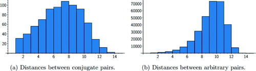
Fig. 10 Histogram of distances between 1000 randomly sampled pairs of arbitrary and conjugate vertices for the prime $p=1,000,003$.

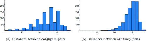
Fig. 11 Proportions of vertex pairs that are opposite; x-axis represents primes. The data are for a random sample of 1000 pairs of conjugate and arbitrary pairs.

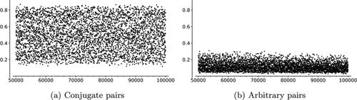
Fig. 12 The horizontal axes of these figures are primes. The heights are proportions of 1000 pairs of arbitrary vertices which are opposite, normalized by $\left|\mathcal{S}\right|$.

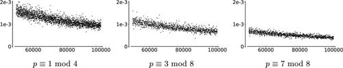
Fig. 13 Normalized proportion of pairs with a shortest path through the specified subgraph, as p varies.

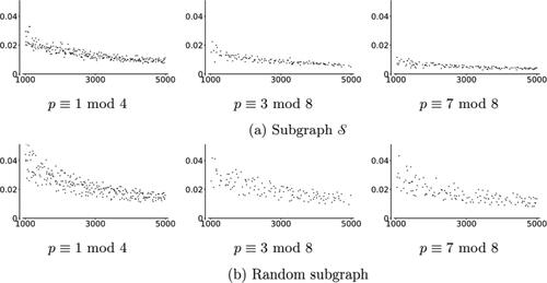
Fig. 14 Distances to the spine $\mathcal{S}$ contrasted with distances to a random subgraph R of the same size. The spine $\mathcal{S}$ is connected for p = 19, 991 and a union of disconnected edges for p = 19, 993.

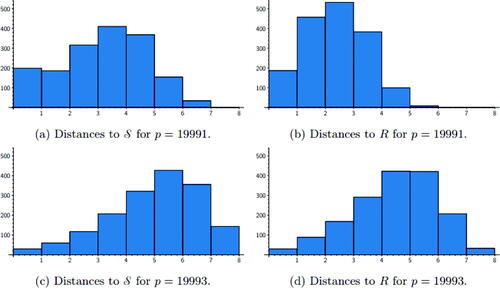
Fig. 15 Normalized average distances d_p to the spine $\mathcal{S}$, as prime p varies on the horizontal axes.

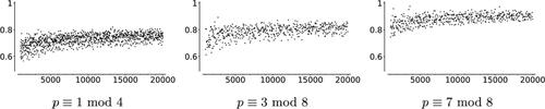
Fig. 16 Size of the spine as prime p varies on the horizontal axes.

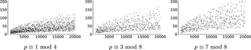
Fig. 17 Proportion of 2-isogenous conjugate pairs in ${\mathcal{G}}_2({\overline{\mathbb{F}}}_p)$ for $10,007\le p\le 100,193.$

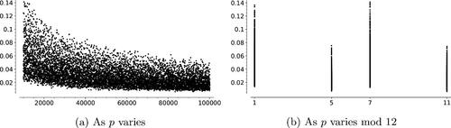
Table 2 Proportions of 2-isogenous conjugates, $10007\le p\le 100193$, sorted by $p\text{mod}12$.

	$p\equiv 1\text{mod}12$	$p\equiv 5\text{mod}12$
Total # of primes:	2079	2104
Mean:	0.043551	0.021969
Standard deviation:	0.019815	0.010206
	$p\equiv 7\text{mod}12$	$p\equiv 11\text{mod}12$
Total # of primes:	2101	2094
Mean:	0.043375	0.022244
Standard deviation:	0.020140	0.010512

Fig. 18 Proportion of 3-isogenous conjugate pairs in ${\mathcal{G}}_2({\overline{\mathbb{F}}}_p)$ for $10,007\le p\le 10,0193.$

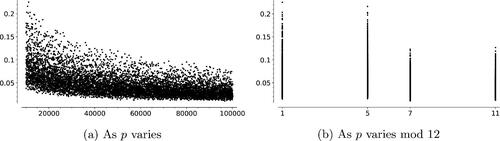
Table 3 Proportions of 3-isogenous conjugates for $10007\le p\le 100193$, sorted by $p\text{mod}12.$

	$p\equiv 1\text{mod}12$	$p\equiv 5\text{mod}12$
Total # of primes:	2079	2104
Mean:	0.058526	0.059034
Standard deviation:	0.029488	0.029729
	$p\equiv 7\text{mod}12$	$p\equiv 11\text{mod}12$
Total # of primes:	2101	2094
Mean:	0.035620	0.036107
Standard deviation:	0.016369	0.016706

Fig. 19 Diameter of ${\mathcal{G}}_2({\overline{\mathbb{F}}}_p)$ for 4600 primes p with $1009\le p\le 9,501,511$ with $y={\hspace{0.17em}\text{log}\hspace{0.17em}}_2(p/12)+1+{\hspace{0.17em}\text{log}\hspace{0.17em}}_2(12)$ (dashed), $y=4/3{\hspace{0.17em}\text{log}\hspace{0.17em}}_2(p/12)+1$ (solid) and the proven lower bound $y={\hspace{0.17em}\text{log}\hspace{0.17em}}_2(p/12)-{\hspace{0.17em}\text{log}\hspace{0.17em}}_2(3)+1$ (dotted).

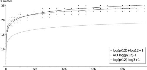
Fig. 20 Lower bounds on the diameter of ${\mathcal{G}}_2({\overline{\mathbb{F}}}_p)$ for 431 primes $p\equiv 23\text{mod}24$ with $1020431<p<15201671$, along with the graphs of $y={\hspace{0.17em}\text{log}\hspace{0.17em}}_2(p/12)+\alpha$ (dashed), $y=4/3{\hspace{0.17em}\text{log}\hspace{0.17em}}_2(p/12)+\beta$ (solid).

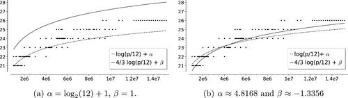
Fig. 21 Diameters of 2-isogeny graph over ${\overline{\mathbb{F}}}_p$ for different congruence classes of the prime p, shown with $y={\hspace{0.17em}\text{log}\hspace{0.17em}}_2(p/12)+{\hspace{0.17em}\text{log}\hspace{0.17em}}_2(12)+1$

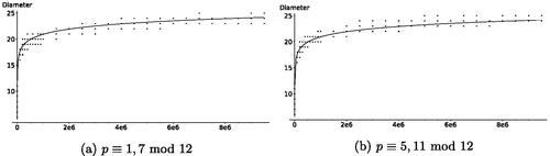
Table 4 Average diameters sorted by primes modulo 12.

average diameter for $100,000<p<300,000$
$1\text{mod}12$	17.2190476190476	$5\text{mod}12$	17.8761061946903
$7\text{mod}12$	17.7346938775510	$11\text{mod}12$	17.9919354838710
average diameter for $300,000<p<500,000$
$1\text{mod}12$	18.4000000000000	$5\text{mod}12$	18.9230769230769
$7\text{mod}12$	18.8235294117647	$11\text{mod}12$	19.1000000000000