Figures & data
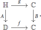
Fig. 1 The gap between
and
in the image of
.
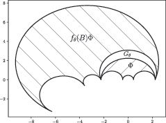
Fig. 2 Domain Ω.
Fig. 3 The crosses represent values of parameters of a disk automorphism estimated using smaller 100-point polygonal approximations
to Ω. The circles are the estimates of λA
and aA
obtained from
.
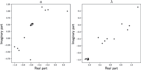
Fig. 4 The crosses represent values of parameters of a disk automorphism estimated using smaller 100-point polygonal approximations
to Ω. The circles are the estimates of λB
and aB
obtained from
.
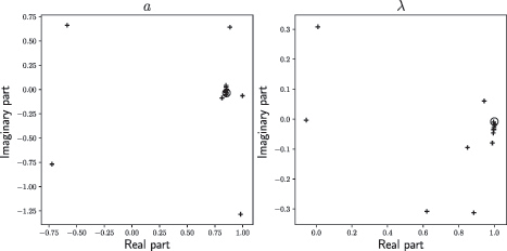
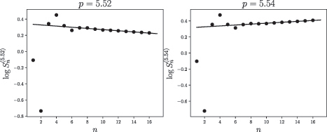
Fig. 5 The plot of as a function of n for
. The solid line is the least-squares best linear fit to the shown data points.
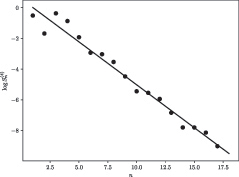
Fig. 6 The plots of as a function of n for
and
. The solid lines are the least-squares best linear fits to the data points
for
, for
.