An Algorithm to Find Ribbon Disks for Alternating Knots

Figures & data

Figure 1: The stevedore knot is algorithmically ribbon. Crossings which make each diagram nonalternating are marked with an asterisk.

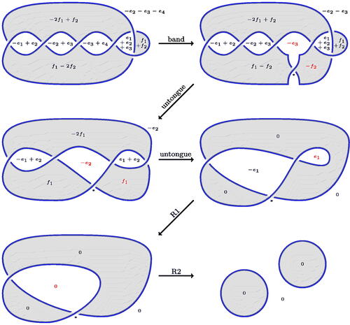
Figure 2: Coloring conventions. An alternating and a nonalternating crossing.

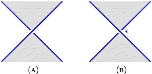
Figure 3: Candidate algorithmic bands. For the length-one band, the twist is chosen such that the new crossing is non-alternating; for the length-two band, one of the two crossings will be non-alternating, depending on the chessboard coloring of the diagram and whether the band crosses over or under.

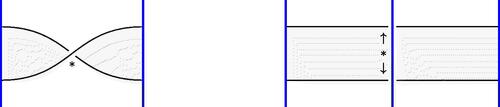
Figure 4: Flype. Here $\sum v$ (resp., $\sum w$) is a sum over all the white (resp., black) regions in the tangle. Vectors associated to white regions in the tangle are multiplied by $-1$ in this move; vectors associated to black regions in the tangle are unchanged. Note also that a special case of the flype is to move a connected summand past a crossing.

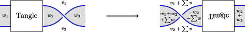
Figure 5: Reidemeister moves preserving bifactorizability. Note that both moves preserve the sum of number of diagram components plus number of nonalternating crossings. Note also that Reidemeister 3 moves change the number of nonalternating crossings and do not preserve bifactorizability.

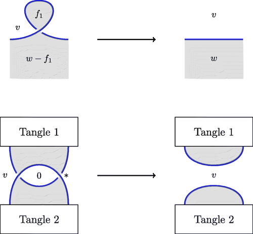
Figure 6: Untongue move.

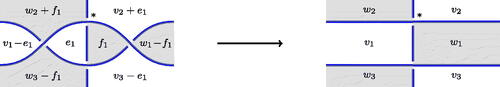
Figure 7: Almost-alternating clasp move.

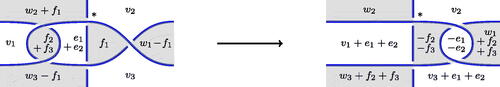
Figure 8: Untongue-2 move.

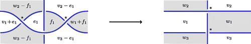
Figure 9: The 3-flype move. Here $\sum v$ (resp., $\sum w$) is a sum over all the white (resp., black) regions in the tangle. Vectors associated to white regions in the tangle are multiplied by $-1$ in this version of the move; black regions in the tangle are unchanged.

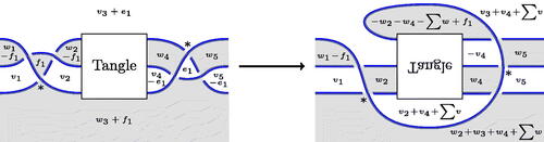
Figure 10: Regions around a band.

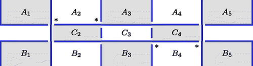
Figure 11: Regions around bands of length three.

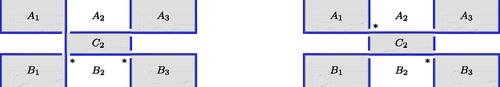
Figure 12: An uninteresting band of length three.

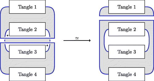
Figure 13: Regions around a band of length one. The horizontal arc is the core of the band.

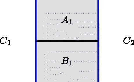
Figure 14: Two-bridge links and ribbon surfaces. Here s and t can be any nonnegative integers, while [[INLINE GRAPHIC]] and $m/(m-q)=[b_1,\dots ,b_l]$.

Figure 15: Algorithmic ribbon surfaces for 2-bridge knots and links, family (d). For s even, there is a minor modification to make in the fourth diagram. Note that one can easily obtain the bifactorizations for each diagram by working back from the crossingless diagram at the bottom.

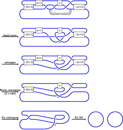
Figure 16: An alternating diagram of $-L\#L$. The tangle marked $\overline{\Gamma }$ is the image of the tangle marked $\Gamma$ under reflection in a plane perpendicular to the plane of the diagram.

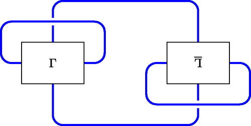
Figure 17: Local contributions to lattice embeddings. The orientation on the overcrossing comes from that on $-L\#L$.

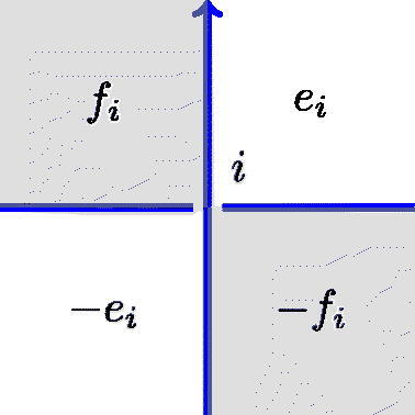
Figure 18: A band move. This is equivalent to composing a length two algorithmic band placed above or below the horizontal strand with an untongue move.

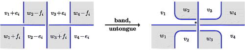
Figure 19: The result of band moves on $-L\#L$. The tangle marked $\overline{{\Gamma }^{\prime }}$ is the image of the tangle marked ${\Gamma }^{\prime }$ under reflection in a plane. After $n-1$ band moves, the tangles ${\Gamma }^{\prime }$ and $\overline{{\Gamma }^{\prime }}$ are crossingless.

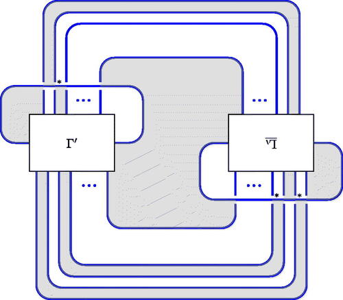
Figure 20: The “floating loop” 3-flype move.

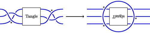
Table 1: Computational results of the Algorithm.

crossings	Prime Alternating Knots	Square Determinant	Bifactorizable	AR	Bands
to 11	563	36	28	28	$1^{28}$
12	1228	62	51	48	$1^{47}\cdot 2^1$
13	4878	175	138	118	$1^{118}$
14	19,536	567	409	305	$1^{301}\cdot 2^4$
15	85,263	1921	1245	850	$1^{805}\cdot 2^{45}$
16	379,799	6888	3724	2330	$1^{2,033}\cdot 2^{297}$
17	1,769,979	24,828	11,259	6513	$1^{5,384}\cdot 2^{1,129}$
18	8,400,285	91,486	34,197	19,071	$1^{13,731}\cdot 2^{5,333}\cdot 3^7$
19	40,619,385	349,453	99,429	52,325	$1^{35,270}\cdot 2^{17,039}\cdot 3^{16}$
20	199,631,989	1,322,355	287,923	150,408	$1^{87,623}\cdot 2^{62,301}\cdot 3^{484}$
21	990,623,857	5,258,538	864,649	430,907	$1^{225,985}\cdot 2^{203,320}\cdot 3^{1,602}$
Total	1,241,536,199	7,056,273	1,303,024	662,903	$1^{371,325}\cdot 2^{289,469}\cdot 3^{2,109}$

In the rightmost column, $a^b$ indicates that b of these knots have algorithmic ribbon disks with not less than a band moves.

Figure 21: Escape bands.

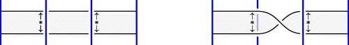
Table 2: Escapees identified and unresolved knots remaining.

Crossings	Non-AR	Obstructed	Candidates	Escapees	Bands	Unresolved
12	3	2	1	1	$2^1$
13	20	20
14	104	100	3	3	$2^3$
15	395	394	1	1	$2^1$
16	1394	1365	29	23	$2^{23}$	6
17	4746	4699	47	46	$2^{46}$	1
18	15,126	14,999	127	91	$2^{91}$	36
19	47,104	46,795	309	262	$2^{257}\cdot 3^5$	47
20	137,515	136,537	978	482	$2^{480}\cdot 3^2$	496
21	433,742	430,231	3511	821	$2^{814}\cdot 3^7$	2690
Total	640,149	635,141	5006	1730	$2^{1,716}\cdot 3^{14}$	3276