A Numerical Stability Analysis of Mean Curvature Flow of Noncompact Hypersurfaces with Type-II Curvature Blowup: II

Figures & data

Figure 1: A MCF solution forming a degenerate neckpinch at spatial infinity with the curvature at the tip (on the left) blowing up at a Type-II rate [2–3].

Figure 2: Numerical simulation of a MCF solution in the Near Class. Rotating each colored curve around the z-axis generates the hypersurface at the corresponding time. (The coordinates z and r are defined on page 3 below.) As the Type-II singularity develops, the dimple disappears.

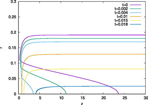
Figure 3: Numerical simulation of a MCF solution in the Far Class. Rotating each colored curve around the z-axis generates the hypersurface at the corresponding time. As the Type-I singularity develops, the dimple becomes a neckpinch.

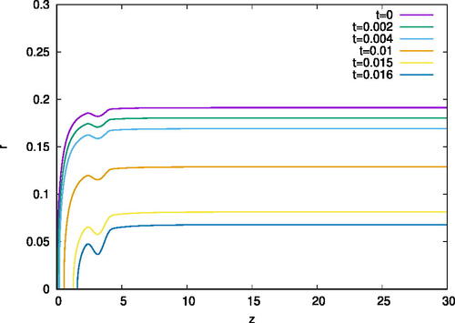
Figure 4: A simulated three-dimensional graph of angular dependent initial embedding for Near Class initial data in a neighborhood of the tip.

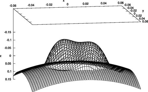
Figure 5: A colored heat map of the initial data represented in Figure 4. The colors correlate with the graph height.

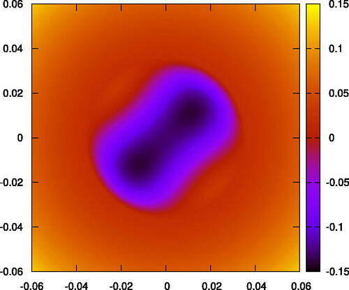
Figure 6: A colored heat map of the mean curvature flow of the initial data depicted in Figure 5. It is clearly becoming rounder.

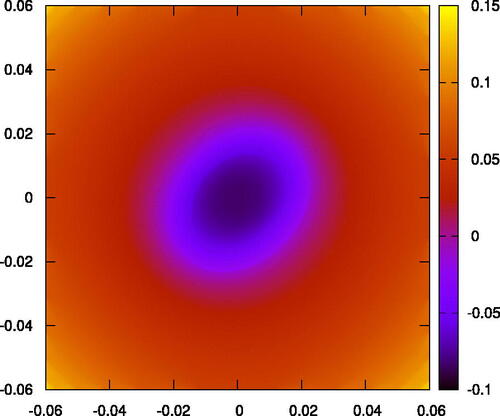
Figure 7: A colored heat map of the mean curvature flow with initial data from Figure 5 at a later time. This time, the angular dependence is gone.

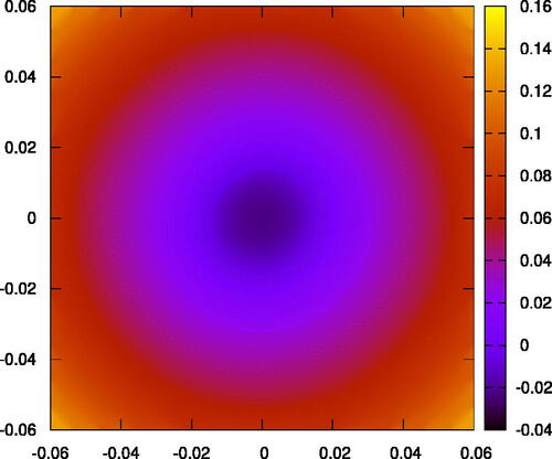
Figure 8: Vertical cross-sections of the mean curvature flow for Far Class initial data at successive times, with $\hspace{0.17em}\cos \hspace{0.17em}(2\theta )$ angular dependence. These cross-sections are chosen to be the location of the developing neck pinch. The loss of the angular dependence is evident.

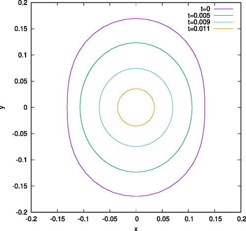
Figure 9: Vertical cross-sections of the MCF for the same initial data in Figure 8, but with the cross-sections obtained to the left of the neck pinch.

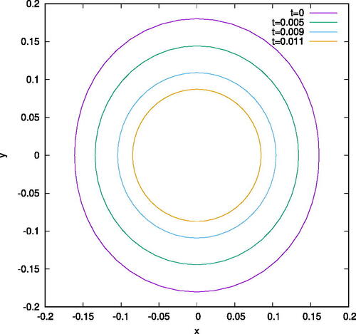
Figure 10: Vertical cross-sections of the MCF for the same initial data in Figure 8, with the cross-sections obtained to the right of the neck pinch.

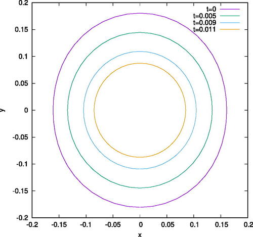
Figure 11: Vertical cross-sections similar to Figure 8, but with imposed angular dependence of $\hspace{0.17em}\cos \hspace{0.17em}(4\theta )$.

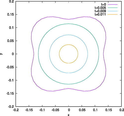
Figure 12: Vertical cross-sections similar to Figure 9, with imposed angular dependence $\hspace{0.17em}\cos \hspace{0.17em}(4\theta )$.

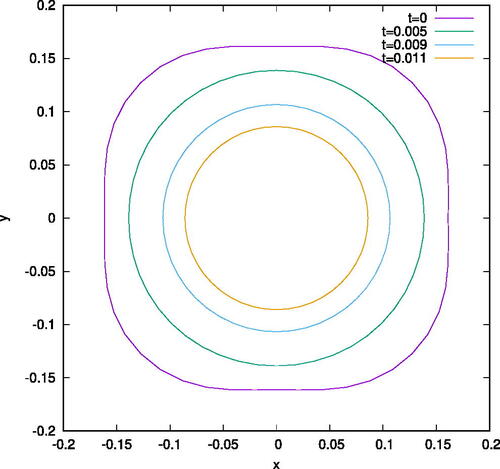
Figure 13: Vertical cross-sections similar to Figure 10, with imposed angular dependence $\hspace{0.17em}\cos \hspace{0.17em}(4\theta )$.