Case depth evaluation of induction-hardened camshaft by using magnetic Barkhausen noise (MBN) method

Figures & data

Figure 1. An illustration shows (a) an alternating sinusoidal magnetic field (black) and the corresponding Barkhausen signal (red), and (b) the rectified Barkhausen bursts during (i) ascending magnetic field excitation and (ii) descending magnetic field excitation

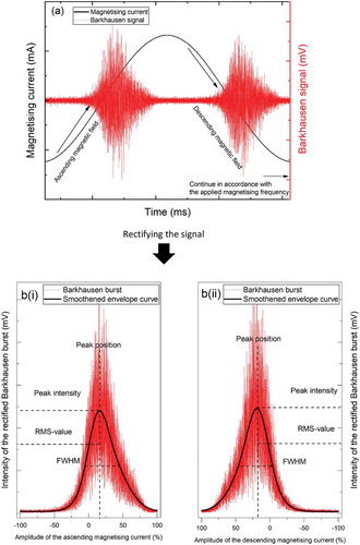
Figure 2. Data from process monitoring of induction-hardened case depth of the cam lobes by means of MBN method

Table 1. Chemical composition of the DIN 17,212 grade CF53N carbon steel

	Fe	C	Al	Si	P	S	Cr	Mn
wt. %	Bal.	0.520–0.560	0.015–0.040	0.150–0.350	0.000–0.025	0.015–0.035	0.100–0.250	0.400–0.700

Figure 3. A schematic diagram shows the Barkhausen measurements (a) in the production line and (b) in the laboratory

Figure 4. Cross-sectional metallography of a qualified induction-hardened component: (a) an optical micrograph; (b) the uppermost martensite layer (0.0 – ~1.0 mm deep); (c) the mixed martensite and bainite in the upper alternating layer (~2.0 mm deep); (d) the mixed bainite, pearlite, martensite and ferrite in the low alternating layer (~4.0 mm deep); (e) the pearlite-ferrite inner core (~5.0 mm deep)

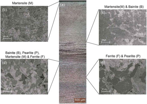
Figure 5. The smoothened envelopes of the rectified Barkhausen bursts obtained during (a) ascending magnetic field excitation and (b) descending magnetic field excitation of the CF53N steel in different heat-treated forms, i.e. pure martensite (Sample A), the bainite-pearlite-martensite-ferrite mixture (Sample B) and the pearlite-ferrite mixture (Sample C)

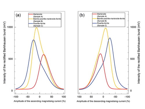
Figure 6. Pulse height distribution of the MBN signals from pure martensite (Sample A), the mixed bainite-pearlite-martensite-ferrite (Sample B) and the mixed pearlite-ferrite (Sample C)

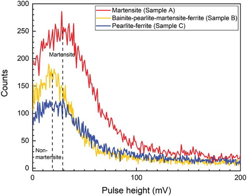
Figure 7. Amplitude spectra from the MBN measurements from pure martensite (Sample A), the mixed bainite-pearlite-martensite-ferrite (Sample B) and the mixed pearlite-ferrite (Sample C)

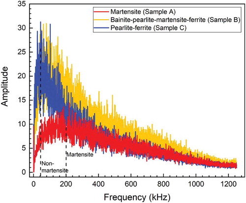
Table 2. Classification of different surface conditions after the induction hardening process

Surface conditions	Criteria
Coarse martensite (×)	Surface layer consists of martensite alone, and the average grain size is > 50 µm
Fine martensite < 3 mm (o)	Surface layer consists of martensite alone, and the average grain size is < 50 µm, with case depth less than 3 mm below and at lower specification limit (LSL)
Fine martensite 3–6 mm (∙)	Surface layer consists of martensite alone, and the average grain size is < 50 µm, with case depth 3–6 mm and within specification range
Non-martensite (*)	Surface layer do not consist of martensite only, but mixtures of martensite, bainite, pearlite and ferrite

Table 3. Parametric features of the Barkhausen measurements from different induction-hardened surface conditions

	Coarse martensite (×)	Fine martensite in layer between 3.0–6.0 mm thick (∙)	Fine martensite in layer < 3.0 mm thick (o)	Non-martensite (*)
Case depth (mm)	> 6.0	3.0–6.0	0.0–2.5	0.0–2.0
mp	115–130	30–60	25–35	30–130
RMS (mV)	450–600	100–400	90–170	200–800
FWHM of the burst (%)	30–35	30–45	35–45	45–65
Peak position in the burst during ascending magnetic field excitation (%)	16–18	14–22	16–21	9 – −11
Peak position in the burst during descending magnetic field excitation (%)	17–19	17–22	16–23	10 – −12
Average peak position in the bursts (%)	16–19	14–22	16–23	10 – −10

Figure 8. Plots of case depth vs. (a) mp and (b) the peak position of the Barkhausen burst stratify on microstructural classifications

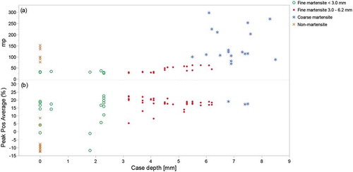
Table 4. Decision criteria (DC) based on the Barkhausen burst characteristics for induction-hardened surface classification

Decisioncriteria (DC)	Leaf label	Average case depth [mm]	Count
1	12.4 ≤ Peak Pos Average (%) < 19.54 and mp < 37.8	1.97	9
2	Peak Pos Average (%) ≥ 21.1 and mp <37.8	2.94	5
3	19.54 ≤ Peak Pos Average (%) < 21.1 and mp < 37.8	3.76	7
4	Peak Pos Average (%) ≥ 12.4 and mp ≥ 37.8 and RMS ≥ 467.85	6.90	12
5	Peak Pos Average (%) ≥ 12.4 and RMS < 467.85 and 37.8 ≤ mp < 61.8	5.33	11
6	Peak Pos Average (%) ≥ 12.4 and RMS < 467.85 and 61.8 ≤ mp	5.80	5
7	Peak Pos Average (%) < 12.4 and RMS ≥ 150.52	0.00	14
8	Peak Pos Average (%) < 12.4 and RMS < 150.52	2.26	5

Figure 9. Data splitted into two random sub-sets, i.e. training (75 %) and validation (25 %), for statistical modelling

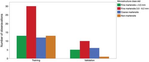
Figure 10. Results of the regression decision tree analysis using the partition platform in JMP Pro®. (a) A statistical overview after 7 splits; (b) summary of the decision tree model; (c) statistical figures of each branch in the decision tree model; (d) a predictive plot of the induction-hardened case depth based on the decision tree model

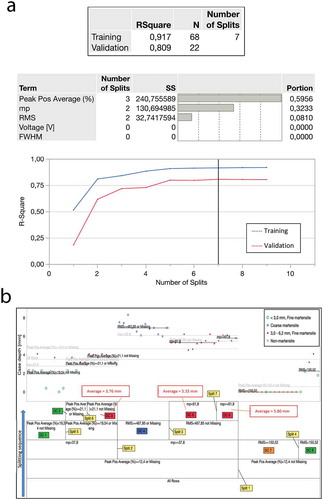
Figure 10. (Continued)

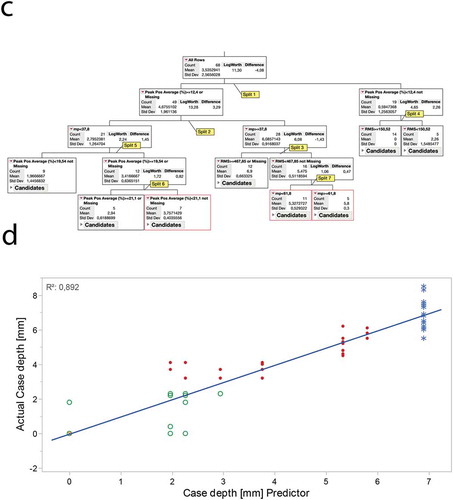
Figure 11. Cross-section morphology of induction-hardened layer with different finishing: (a) uniform layer; (b) non-uniform layer

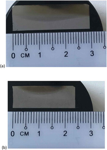
Figure 12. Comparison between (a) the COMSOL numerical model and (b) the in-line data