
Figures & data
Figure 1. Drawings of RC column-footing subassembly test specimens: (a) Elevation view (Specimen 1 and 2), (b) Cross section (Specimen 1 and 2), and (c) lap splice detail Specimen 2. All dimensions in (mm).
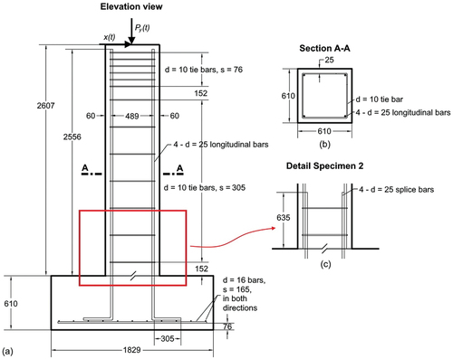
Figure 2. Loading protocol for (a) Specimen 1 and (b) Specimen 2: Applied lateral displacement, x(t) (green lines) and vertical load, Py(t) (grey lines). Vertical black dotted lines with numerical values denote the displacement ductility level, μ.
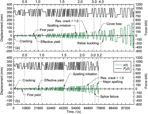
Figure 3. Illustrations of test specimen showing GPR/UEA scan lines and sample final reconstructed images: (a) Isometric view from north-east and (b) elevation view of column west face. N = north, S = south, E = east, and W = west. All dimensions in (mm).
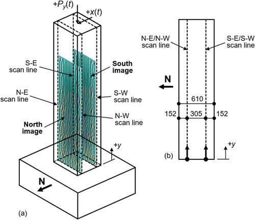
Figure 4. Illustration of image reconstruction and fusion methodology. N = north, S = south, E = east, and W = west.
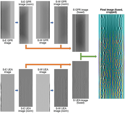
Figure 5. Load-drift response of (a) Specimen 1 and (b) Specimen 2.
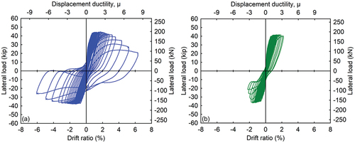
Figure 6. Sample final fused images Specimen 1 (South): (a) Baseline image (μ = 0) and (b) image at ductility level, μ = 2.0. Column width, d = 610 mm. The location and dimensions of the three designated damage regions are shown in Figure 7. Final images for both specimens and additional ductility levels can be found in Appendix, Figures A1 through A4.
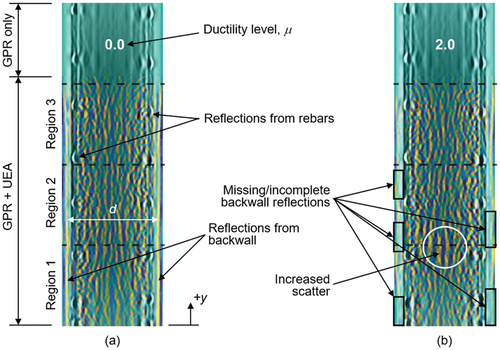
Figure 7. Illustrations of (a) applied loads, (b) and (c) internal force curves (qualitative), (d) elevation view of specimen north face with sample final reconstructed image and three designated damage regions, and (e) photo of sample specimen during testing with highlighted cracks (red lines) and designated damage regions (dashed black lines). All dimensions in (mm).
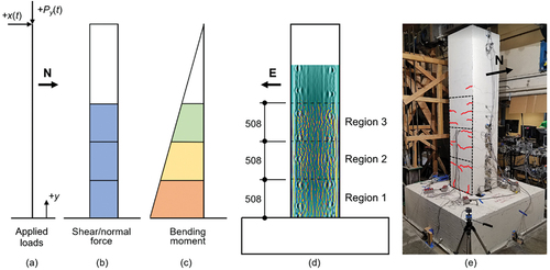
Figure 8. SSIM curves for (a) Specimen 1 and (b) Specimen 2. The dashed horizontal lines at 0.5 and 0.25 are provided for reference (locations arbitrary).
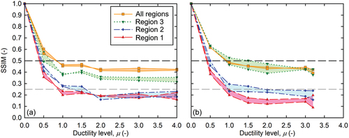
Figure 9. SSIM curves for GPR, UEA, and fused images (for Specimen 2, north image). The dashed horizontal lines at 0.5 and 0.25 are provided for reference (locations arbitrary).
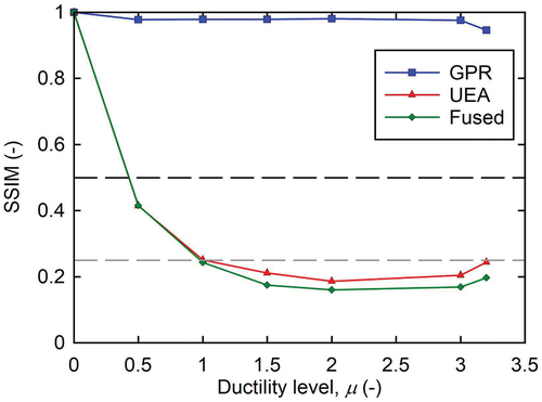
Figure 10. Illustration of the tracked backwall amplitude bands for Specimen 2, south side. Mean values within the blue and red bands are used in the backwall analysis.
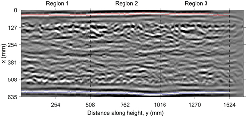
Figure 11. Average normalized backwall amplitude curves per damage region for (a) Specimen 1 and (b) Specimen 2. The values plotted here correspond to the numbers shown in red in Appendix, Figures A5 and A6.
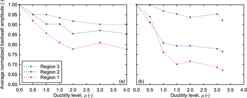
Figure A1. Reconstructed images specimen 1, south scan: (a) to (g) correspond to ductility levels, μ = 0.0 (= Baseline) to 4.0, respectively (also shown above region 3). The location and dimensions of the three designated damage regions are shown in Figures 6 and 7.
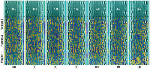
Figure A2. Reconstructed images specimen 1, north scan: (a) to (g) correspond to ductility levels, μ = 0.0 (= Baseline) to 4.0, respectively (also shown above region 3). The location and dimensions of the three designated damage regions are shown in Figures 6 and 7.
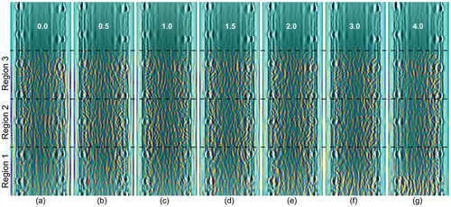
Figure A3. Reconstructed images specimen 2, south scan: (a) to (g) correspond to ductility levels, μ = 0.0 (= Baseline) to 3.2, respectively (also shown above region 3). The location and dimensions of the three designated damage regions are shown in Figures 6 and 7.
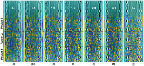
Figure A4. Reconstructed images specimen 2, north scan: (a) to (g) correspond to ductility levels, μ = 0.0 (= Baseline) to 3.2, respectively (also shown above Region 3). The location and dimensions of the three designated damage regions are shown in Figures 6 and 7.
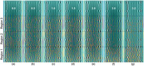
Figure A5. Mean backwall amplitude envelopes from all four images for specimen 1. Red lines and numbers represent the average value across each region. The numbers on top denote the ductility level, μ.
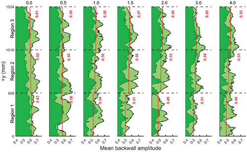
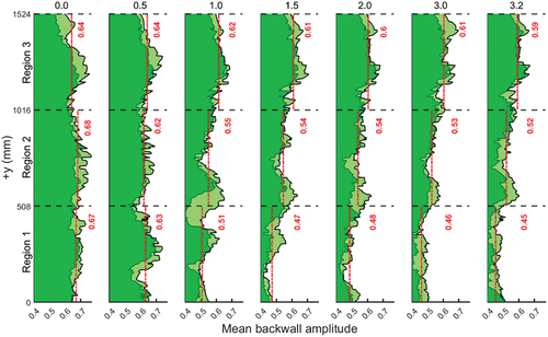
Figure A6. Mean backwall amplitude envelopes from all four images for specimen 2. Red lines and numbers represent the average value across each region. The numbers on top denote the ductility level, μ.
Data availability statement
The data that support the findings of this study are available from the corresponding author, TS, upon reasonable request.