Numerical Simulations and Design Optimization of Compressor Cascade Flow Using One Equation and Wray-Agarwal Turbulence Model

Figures & data

Table 1. Constants used in WA turbulence model.

Constant Symbols	Value
$C_{1k\omega }$	0.0829
$C_{1kϵ}$	0.1127
$C_1$	$f_1(C_{1k\omega }-C_{1kϵ})+C_{1kϵ}$
${\sigma }_{k\omega }$	0.72
${\sigma }_{kϵ}$	1.0
${\sigma }_R$	$f_1({\sigma }_{k\omega }-{\sigma }_{kϵ})+{\sigma }_{kϵ}$
$C_{2k\omega }$	${\displaystyle \frac{C_{1k\omega }}{{\kappa }^2}}+{\sigma }_{k\omega }$
$C_{2kϵ}$	${\displaystyle \frac{C_{1kϵ}}{{\kappa }^2}}+{\sigma }_{k\omega }$
$\kappa$	0.41
$C_{\omega }$	8.54

Table 2. Key parameters of compressor cascade.

Parameter	Value
Chord length	150.00 mm
Span length	370.00 mm
Solidity	1.12
Stagger angle	42.70°
Camber angle	23.22°
Aspect ratio	2.47
Design upstream flow angle	54.31°
Design downstream flow angle	31.09°
Inlet velocity magnitude	40.00 m/s

Figure 1. Computational domain and boundary conditions of compressor cascade.

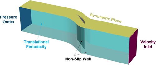
Figure 2. Inlet velocity profile in computational domain.

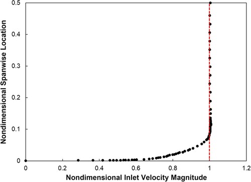
Figure 3. Study of mesh size on solution and relative error.

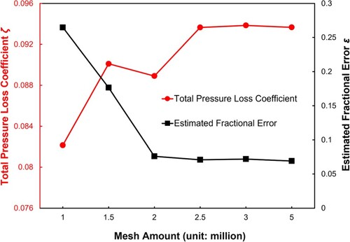
Figure 4. Mesh generated inside the compressor cascade passage (2.5 Million): (a) 3D passage mesh, (b) 2D cascade mesh.

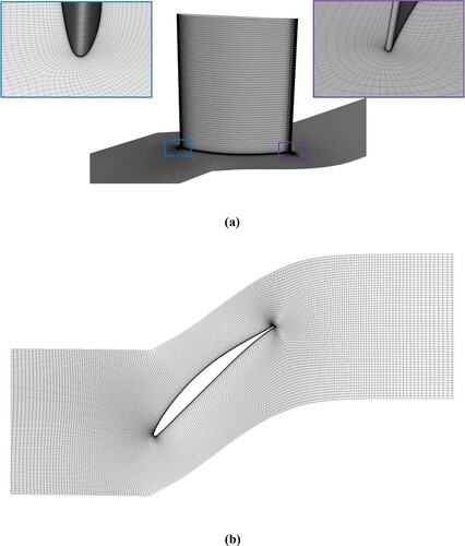
Figure 5. Near-wall static pressure coefficients at two different span-wise stations at incidence angle of 0 degree at (a) 5.4% span-wise station, and (b) 50% span-wise station (mid-span).

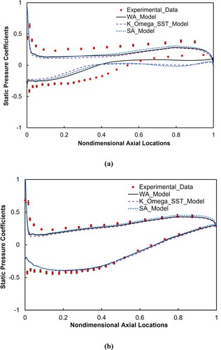
Figure 6. Total pressure loss coefficients downstream of compressor cascade at incidence angle of 0 degree: (a) contours of total pressure loss coefficient downstream of compressor cascade, and (b) span-wise distributions of circumferentially averaged total pressure loss coefficients.

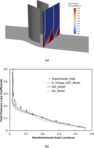
Figure 7. Near-wall static pressure coefficients at two different span-wise sections at incidence angle of 2 degrees at (a) 5.4% span-wise section, and (b) 50% span-wise section.

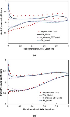
Figure 8. Total pressure loss coefficients downstream of compressor cascade at incidence angle of 2 degrees: (a) contours of total pressure loss coefficient downstream of cascade, and (b) span-wise distributions of circumferentially averaged total pressure loss coefficients.

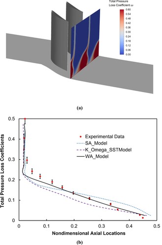
Figure 9. Near-wall pressure coefficients at four different span-wise sections at incidence angle of 4 degree at (a) 1.4% span-wise section, (b) 5.4% span-wise section, (c) 16.2% span-wise section, and (d) 50% span-wise section coefficients.

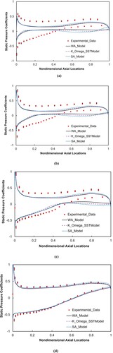
Figure 10. Total pressure loss coefficients downstream of compressor cascade at incidence angle of 4 degrees (a) contours of total pressure loss coefficient downstream cascade, and (b) distributions of circumferentially averaged total pressure loss coefficients.

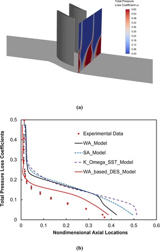
Figure 11. Flowchart of adjoint optimisation process.

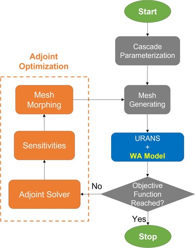
Figure 12. Contours of sensitivity value.

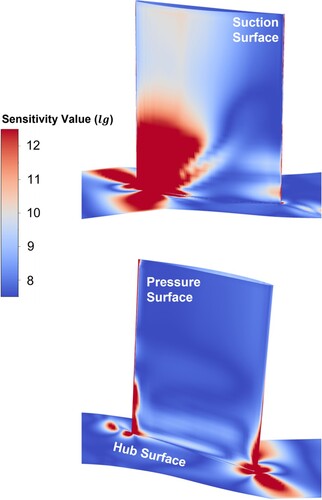
Figure 13. Comparison of cascade airfoil profiles near the hub region.

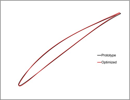
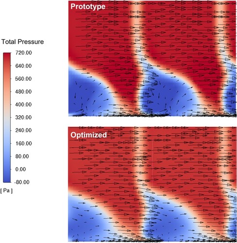
Figure 14. Flowfield comparison between prototype and optimised compressor cascade passage.