2,357
Views
27
CrossRef citations to date
0
Altmetric
Robust Stats, Outliers, Image Analysis, Nonparametric

A Measure of Directional Outlyingness With Applications to Image Data and Video

, &
Pages 345-359 | Received 01 Aug 2016, Published online: 17 May 2018

Figures & data

Figure 1. Scale estimates of the family income data. The SDO scale is measured symmetrically about the median, whereas the DO scales are not and reflect skewness.
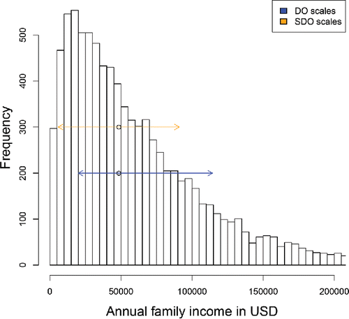
Figure 1. Scale estimates of the family income data. The SDO scale is measured symmetrically about the median, whereas the DO scales are not and reflect skewness.

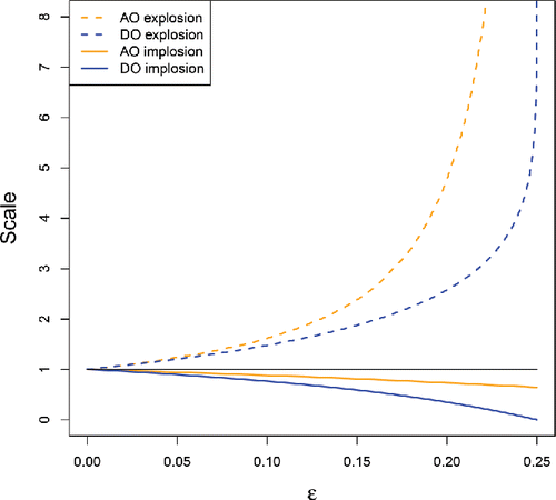
Figure 2. Comparison of explosion and implosion bias of the AO and DO scales.

Figure 2. Comparison of explosion and implosion bias of the AO and DO scales.

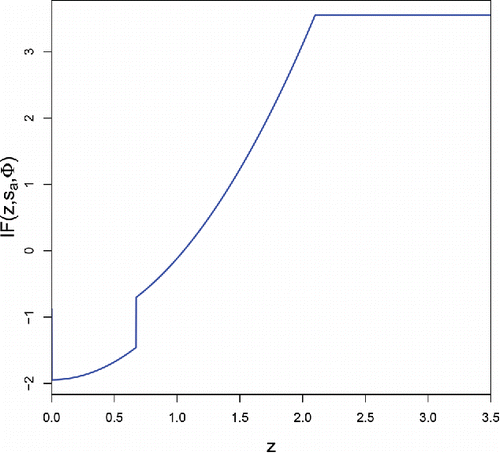
Figure 3. Influence function of sa at F = Φ.

Figure 3. Influence function of sa at F = Φ.

Figure 4. Influence function of DO(x) for F = Φ. Left: 3D, right: 2D seen from above. For a fixed point x it is bounded over all possible positions z of contamination.
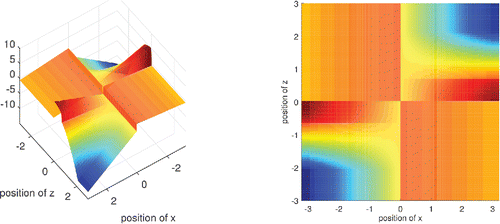
Figure 4. Influence function of DO(x) for F = Φ. Left: 3D, right: 2D seen from above. For a fixed point x it is bounded over all possible positions z of contamination.

Figure 5. Bloodfat data with (a) SDO contours, and (b) DO contours. The DO contours better reflect the skewness in the data.
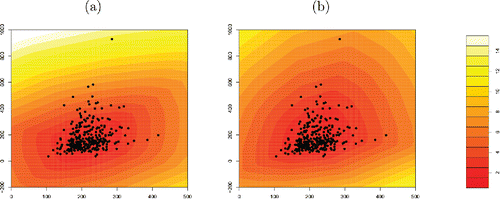
Figure 5. Bloodfat data with (a) SDO contours, and (b) DO contours. The DO contours better reflect the skewness in the data.

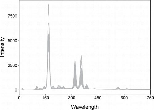
Figure 6. Spectra of 180 archeological glass samples.

Figure 6. Spectra of 180 archeological glass samples.

Figure 7. Functional DO (fDO) values of the 180 glass spectra. Higher fDO values correspond to curves that are more outlying on average.
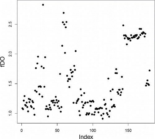
Figure 7. Functional DO (fDO) values of the 180 glass spectra. Higher fDO values correspond to curves that are more outlying on average.

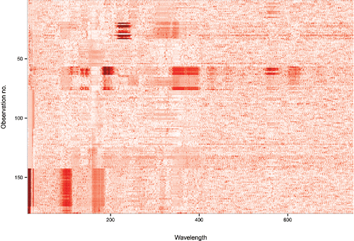
Figure 8. Heatmap of DO of the glass data. Darker pixels indicate outlying behavior.

Figure 8. Heatmap of DO of the glass data. Darker pixels indicate outlying behavior.

Figure 9. Outlier cutoffs for the family income data. The DO-based cutoff takes the data skewness into account.
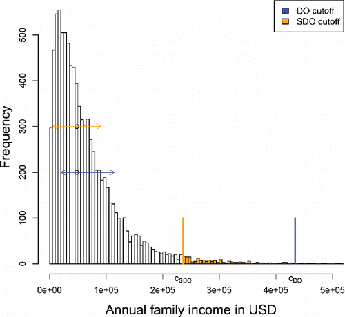
Figure 9. Outlier cutoffs for the family income data. The DO-based cutoff takes the data skewness into account.

Figure 10. Outlier detection on bloodfat data. The DO-based cutoff adapts to the data skewness and flags fewer points as outlying.
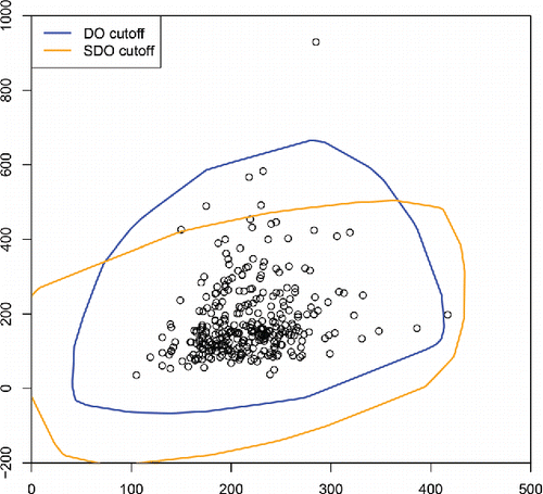
Figure 10. Outlier detection on bloodfat data. The DO-based cutoff adapts to the data skewness and flags fewer points as outlying.

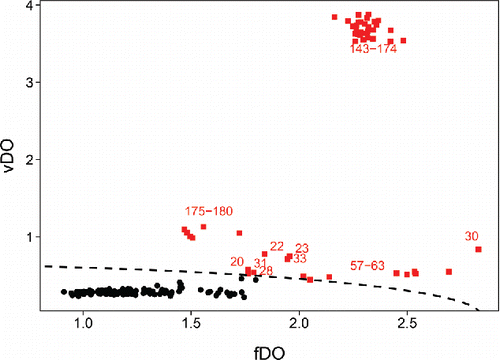
Figure 11. Functional outlier map (FOM) of the glass data, with cutoff curve.

Figure 11. Functional outlier map (FOM) of the glass data, with cutoff curve.

Figure 12. Original MRI image of subject 387, and its derivatives in the horizontal and vertical direction.

Figure 12. Original MRI image of subject 387, and its derivatives in the horizontal and vertical direction.

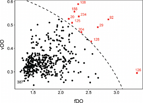
Figure 13. Functional outlier map (FOM) of the MRI dataset, with cutoff curve.

Figure 13. Functional outlier map (FOM) of the MRI dataset, with cutoff curve.

Figure 14. MRI image (left) and DO heatmap (right) of subjects 387 (top), 92 (middle), and 126 (bottom).
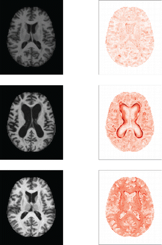
Figure 14. MRI image (left) and DO heatmap (right) of subjects 387 (top), 92 (middle), and 126 (bottom).

Figure 15. Frames number 100, 487, 491, and 500 from the video dataset.

Figure 15. Frames number 100, 487, 491, and 500 from the video dataset.

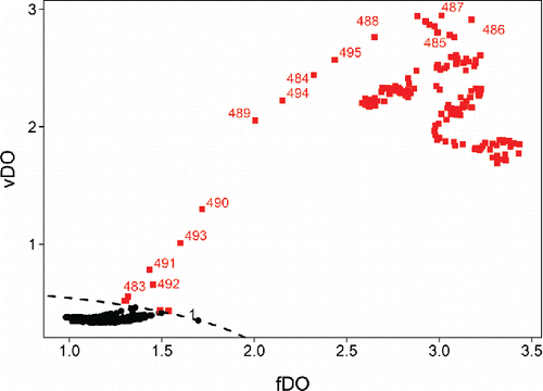
Figure 16. Functional outlier map of the video data.

Figure 16. Functional outlier map of the video data.

Figure 17. Left: Frames 100, 487, 491, and 500 from the video. Middle: DO heatmaps of these frames. Right: FOM with blue marker at the position of the frame.
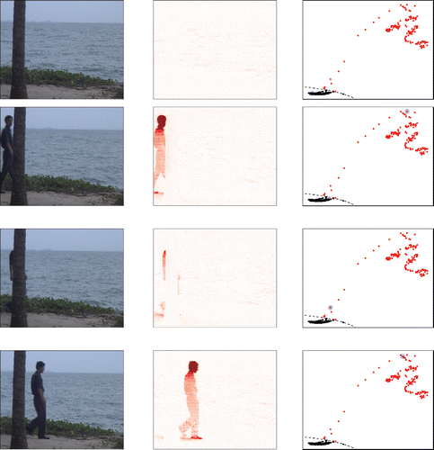
Figure 17. Left: Frames 100, 487, 491, and 500 from the video. Middle: DO heatmaps of these frames. Right: FOM with blue marker at the position of the frame.

Figure 18. Percentage of outliers found in univariate lognormal samples of size n = 200 (left), n = 500 (middle), and n = 1000 (right), with 10% (top) and 15% (bottom) of outliers in x.
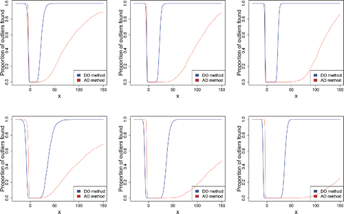
Figure 18. Percentage of outliers found in univariate lognormal samples of size n = 200 (left), n = 500 (middle), and n = 1000 (right), with 10% (top) and 15% (bottom) of outliers in x.

Figure 19. Percentage of outliers found in multivariate skew normal samples of size n = 200 (left), n = 500 (middle), and n = 1000 (right), with 10% of outliers around x=(x,,x)T, in dimensions d = 2 (top), d = 5 (middle), and d = 10 (bottom).
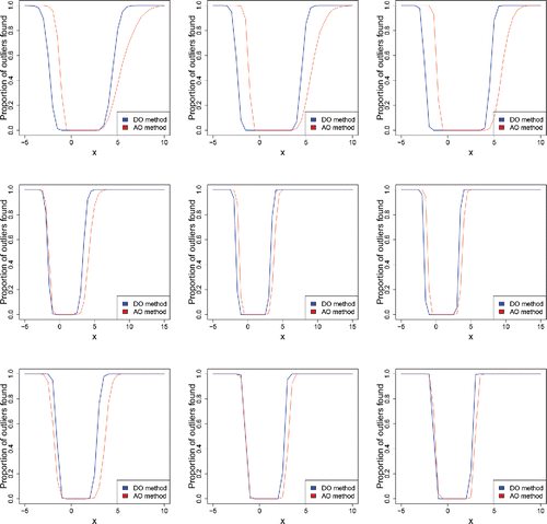
Figure 19. Percentage of outliers found in multivariate skew normal samples of size n = 200 (left), n = 500 (middle), and n = 1000 (right), with 10% of outliers around x=(x,…,x)T, in dimensions d = 2 (top), d = 5 (middle), and d = 10 (bottom).

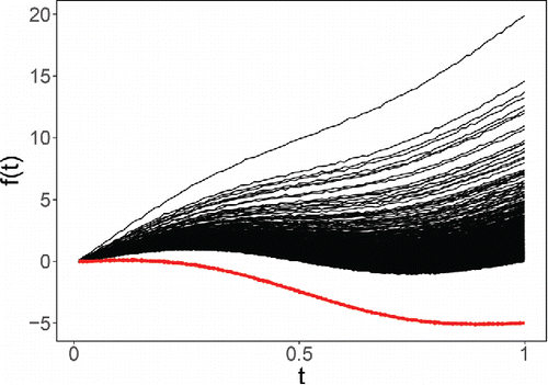
Figure 20. n = 1000 generated functions with 10% contamination.

Figure 20. n = 1000 generated functions with 10% contamination.

Figure 21. Percentage of outliers found in functional samples of size n = 200 (left), n = 500 (middle), and n = 1000 (right), with 10% of contaminated curves with slope L.

Figure 21. Percentage of outliers found in functional samples of size n = 200 (left), n = 500 (middle), and n = 1000 (right), with 10% of contaminated curves with slope L.

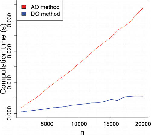
Figure 22. Average computation time of DO and AO as a function of sample size.

Figure 22. Average computation time of DO and AO as a function of sample size.