Adaptive Incremental Mixture Markov Chain Monte Carlo

Figures & data

Table 1 (Example 1) Results for ${\pi }_1$: effective sample size (ESS) (the larger the better), mean squared error (MSE) of ${\pi }_1(X>5)$ (the smaller the better).

	ESS	MSE ($\times {10}^4$)
AMH	$(0.08,0.004)$	6030
AGM-2	$(0.12,0.001)$	120
AGM-3	$(0.51,0.091)$	76
AGM-40	$(0.91,0.008)$	5
AIMM	$(0.47,0.004)$	7

NOTE: Estimates obtained through 100 independent runs of the four methods, each of 20,000 iterations, discarding the first 10,000 iterations for burn in. For the ESS statistic, the mean and variance are provided.

Fig. 1 (Example 1) Illustration of one AIMM increment for the target π₁. Top: States $X_1,\dots ,X_n$ of the AIMM chain, proposed new state ${\tilde{X}}_{n+1}$ activating the increment process (i.e., satisfying $W_n({\tilde{X}}_{n+1})\ge \overline{W}$), and neighborhood of ${\tilde{X}}_{n+1}$, $\mathfrak{N}({\tilde{X}}_{n+1} | X_1,\dots ,X_n)$. Bottom: Target π₁, defensive kernel Q₀, first increment ${\varphi }_1$, and updated kernel Q₁ plotted on a logarithmic scale.

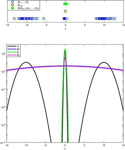
Fig. 2 (Example 1) Illustration of AIMM sampling from the target π₁ for $n=20,000$ iterations sequence of proposals from Q₀ to Q_n produced by AIMM.

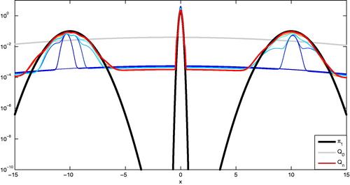
Fig. 3 (Example 2: π₂ target, d = 2) Incremental mixture created by AIMM for three different initial proposals. Top row: Q₀ is a Gaussian density (the region inside the black dashed ellipses contains 75% of the Gaussian mass) centred on a high density region (left) and a low density region (right). Bottom row: Q₀ is Uniform (with support corresponding to the black dashed rectangle). The components ${\varphi }_1,\dots ,{\varphi }_{M_n}$ of the incremental mixture obtained after $n=100,000$ MCMC iterations are represented through (the region inside the ellipses contains 75% of each Gaussian mass). The color of each ellipse illustrates the corresponding component’s relative weight ${\beta }_{\ell }$ (from dark blue for lower weights to red).

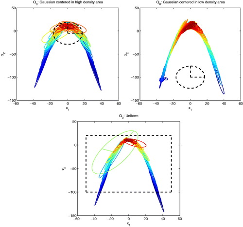
Table 2 (Example 2: π₂ target, d = 2) Influence of the initial proposal Q₀ on AIMM outcome after $n=100,000$ MCMC iterations (replicated 20 times).

Q0	Mn	$\mathit{ESS}$	$\mathit{ACC}$	$\mathit{KL}$	$\mathit{JMP}$	$\mathit{EFF}$ ($\times {10}^{-4}$)
Gaussian on a high density region	41	0.19	0.35	0.59	197	11
Gaussian on a low density region	157	0.23	0.37	0.71	245	4
Uniform on $\mathfrak{S}$	39	0.24	0.38	0.62	320	11

NOTE: M_n is the number of components created by AIMM, $\mathit{ESS}$ is the effective sample size, $\mathit{ACC}$ is the acceptance rate, $\mathit{KL}$ is the KL divergence between ${\pi }_2$ and the chain distribution, $\mathit{JMP}$ is the average distance between two consecutive states of the chain, and $\mathit{EFF}$ is a time-normalized ESS.

Fig. 4 (Example 2: π₂ target, d = 2) AIMM’s incremental mixture design after $n=100,000$ MCMC iterations. (a) Evolution of the number of kernels M_n created by AIMM for different thresholds. (b) Evolution of the KL divergence between ${\pi }_2$ and the incremental proposal Q_n, plotted in lin-log scale.

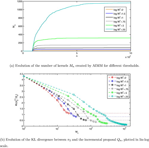
Table 3 (Example 2: π₂ target, d = 2) Influence of the threshold $\overline{W}$ on AIMM and f-AIMM outcomes after $n=100,000$ MCMC iterations (replicated 20 times).

(a) AIMM
$\text{log}\hspace{0.17em}\overline{W}$	Mn	$\mathit{ESS}$	$\mathit{ACC}$	$\mathit{KL}$	$\mathit{JMP}$	$\mathit{CPU}$	$\mathit{EFF}$ $(\times {10}^{-4})$
10	0	0.03	0.01	14.06	10	45	2
2	21	0.16	0.27	0.72	169	154	10
1.5	39	0.24	0.38	0.62	235	245	10
1	79	0.37	0.53	0.54	331	330	12
0.75	149	0.48	0.64	0.53	286	658	7
0.5	317	0.64	0.75	0.51	451	2199	3
0.25	1162	0.71	0.87	0.54	505	6201	1
(b) f-AIMM
$\text{log}\hspace{0.17em}\overline{W}$	$M_{\text{max}}$	$\mathit{ESS}$	$\mathit{ACC}$	$\mathit{KL}$	$\mathit{JMP}$	$\mathit{CPU}$	$\mathit{EFF}$ $(\times {10}^{-4})$
1.5	25	0.29	0.51	0.59	268	255	11
0.75	100	0.53	0.69	0.53	409	421	13
0.5	200	0.67	0.80	0.51	474	1151	6

Fig. 5 (Example 5) Information regarding the acceptance rate of 100 AIMM runs are reported on the left panel and the evolution of the number of components for about 10 runs throughout the sampling is shown on the right panel.

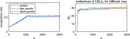
Table 4 (Example 3: π₃ target, d = 6) Comparison of f-AIMM with the four other samplers after $n=200,000$ iterations (replicated 10 times).

	$\overline{W}$	$M_{\text{max}}$	$\mathit{ACC}$	$\mathit{ESS}$	$\mathit{CPU}$	$\mathit{EFF}$	$\mathit{JMP}$
f-AIMM	10	20	0.049	0.015	274	$5.2\times {10}^{-5}$	0.08
f-AIMM	1	70	0.169	0.089	517	$1.7\times {10}^{-4}$	0.27
f-AIMM	0.1	110	0.251	0.156	818	$1.9\times {10}^{-4}$	0.38
RWMH		–	0.23	0.001	109	$9.2\times {10}^{-6}$	0.007
AMH		–	0.42	0.002	2105	$9.5\times {10}^{-7}$	0.004
AGM-MH		100	0.009	0.002	2660	$3.4\times {10}^{-6}$	0.003
IM		–	0.003	0.001	199	$5.5\times {10}^{-6}$	0.003

Table 5 (Example 4: π₄ target, $d\in \{4,10\}$) Comparison of f-AIMM with RWMH, AMH, AGM, and IM after $n=200,000$ iterations (replicated 100 times).

(a) π4 in dimension d = 4
	$\overline{W}$	$M_{\text{max}}$	$\mathit{ACC}$	$\mathit{ESS}$	$\mathit{CPU}$	$\mathit{EFF}$	$\mathit{JMP}$
f-AIMM	5	100	0.69	0.30	408	$7.3\times {10}^{-4}$	68
RWMH		–	0.23	$3.1\times {10}^{-3}$	93	$3.4\times {10}^{-5}$	0.09
AMH		–	0.26	$2.7\times {10}^{-2}$	269	$1.0\times {10}^{-4}$	0.64
AGM-MH		100	$3.0\times {10}^{-3}$	$5.0\times {10}^{-4}$	3517	$1.4\times {10}^{-7}$	0.29
IM		–	$3.3\times {10}^{-4}$	$5.9\times {10}^{-4}$	81	$7.3\times {10}^{-6}$	0.05
(b) π4 in dimension d = 10
	$\overline{W}$	$M_{\text{max}}$	$\mathit{ACC}$	$\mathit{ESS}$	$\mathit{CPU}$	$\mathit{EFF}$	$\mathit{JMP}$
f-AIMM	20	100	0.45	0.18	1232	$1.4\times {10}^{-4}$	116.4
f-AIMM	10	200	0.64	0.25	1550	$1.6\times {10}^{-4}$	200.1
RWMH		–	0.38	$7.2\times {10}^{-4}$	476	$1.7\times {10}^{-6}$	0.07
AMH		–	0.18	$1.3\times {10}^{-3}$	2601	$5.0\times {10}^{-7}$	0.57
AGM-MH		100	$2.6\times {10}^{-4}$	$5.0\times {10}^{-4}$	4459	$1.1\times {10}^{-7}$	$7.1\times {10}^{-3}$
IM		–	$6.4\times {10}^{-5}$	$6.1\times {10}^{-4}$	473	$1.2\times {10}^{-6}$	$4.1\times {10}^{-3}$

Table 6 (Example 4: π₄ target, $d\in \{4,10\}$) Mean square error (MSE) of the mixture parameter λ, for the different algorithms (replicated 100 times).

	$\overline{W}$	$M_{\text{max}}$	$\mathit{MSE}(\lambda ),d=4$	MSE($\lambda$), d = 10
f-AIMM	5	100	0.0001	0.06
f-AIMM	20	100	0.0006	0.09
f-AIMM	10	200	0.0024	0.01
RWMH		–	0.25	0.25
AMH		–	0.15	0.25
AGM-MH		100	0.22	0.25
IM		–	0.03	0.20

Fig. 6 (Example 5) Marginal posterior distribution of three parameters of the model estimated after 70,000 iterations of AIMM.

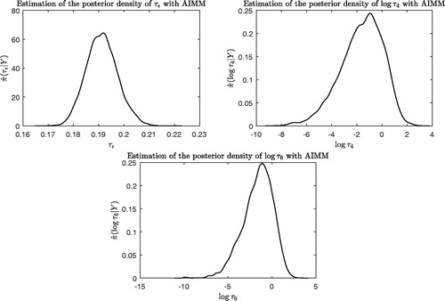
Fig. 7 (Example 6) Marginal posterior of four parameters estimated by AIMM and ARMS after a long run of 100,000 iterations of both algorithm (full swipe update Metropolis-within-Gibbs for ARMS).

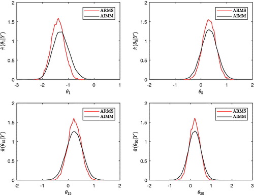
Table 7 (Example 6) Comparison of the performance of three adaptive MCMC samplers: acceptance rate, integrated autocorrelation time and average squared jumping distance.

	Acc rate	IACT	Avg sq. distance ($\times {10}^{-4}$)
AIMM	0.49	1.12	16,203
ARMS	0.53	0.98	11,270
RAMA	0.23	31.6	2.756

NOTE: Results for AIMM and ARMS are estimated based after 10,000 iterations of 100 independent runs (full swipe update Metropolis-within-Gibbs for ARMS). Results for RAMA were reported from (Roberts and Rosenthal 2009, Table p. 360).

Roberts, G. O., and Rosenthal, J. S. (2009), “Examples of Adaptive MCMC,” Journal of Computational and Graphical Statistics, 18, 349–367. DOI:10.1198/jcgs.2009.06134.

 Web of Science ®Google Scholar