Rerandomization Strategies for Balancing Covariates Using Pre-Experimental Longitudinal Data

Figures & data

Fig. 1 The electricity consumption (kWh) during the pretreatment month for the 54 households included in the experiment.

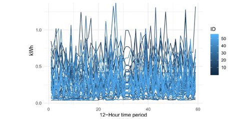
Fig. 2 The cumulative distribution function for the Mahalanobis distance ($\text{df}=3$) of the 800th order statistic in the random sample of allocations for numbers of allocations between 100,000 and 1,000,000.

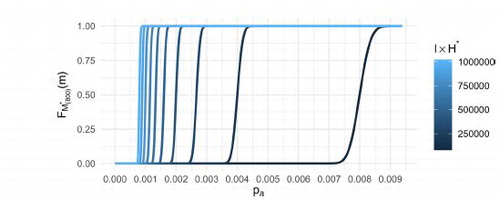
Fig. 3 Relative power as compared to complete randomization for Mahalanobis distance (M) and ranked p-values (R) rerandomization designs. The left and right figures display the results for DGPs A and B, respectively.

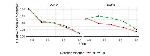
Table 1 Relative variance change in the covariates and the effect estimate as compared to complete randomization (Equations (15)(15) $$\text{VC}(k|d)\equiv \frac{\text{var}({\overline{\mathbf{Z}}}_{kT}-{\overline{\mathbf{Z}}}_{kT}|d)-\text{var}({\overline{\mathbf{Z}}}_{kT}-{\overline{\mathbf{Z}}}_{kT}|c)}{\text{var}({\overline{\mathbf{Z}}}_{kT}-{\overline{\mathbf{Z}}}_{kT}|c)},$$(15) and (16)(16) $${\text{VC}}_{\tau }(d)\equiv \frac{\text{var}({\widehat{\tau }}_d)-\text{var}({\widehat{\tau }}_c)}{\text{var}({\widehat{\tau }}_c)}.$$(16) ) for Mahalanobis distance (M) and ranked p-values (R) rerandomization designs.

	A		B
Balance measure	R	M	R	M
$\text{VC}(X_1|.)$	–0.71	–0.74	–0.83	–0.74
$\text{VC}(X_2|.)$	–0.71	–0.75	–0.83	–0.75
$\text{VC}(X_3|.)$	–0.70	–0.75	–0.73	–0.75
VC τ(.)	–0.20	–0.19	–0.22	–0.20

NOTE: The left and right panels display the results for DGPs A and B, respectively.

Fig. 4 Relative power as compared to complete randomization for Mahalanobis distance (M) and ranked p-values (R) rerandomization designs. The left and right panels display the results including four (K = 4) and eleven (K = 11) covariates, respectively.

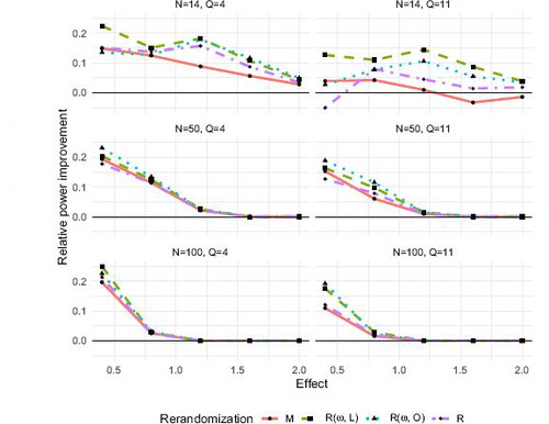
Table 2 Relative change in variance of the covariates and in the effect estimate as compared to complete randomization (Equations (15)(15) $$\text{VC}(k|d)\equiv \frac{\text{var}({\overline{\mathbf{Z}}}_{kT}-{\overline{\mathbf{Z}}}_{kT}|d)-\text{var}({\overline{\mathbf{Z}}}_{kT}-{\overline{\mathbf{Z}}}_{kT}|c)}{\text{var}({\overline{\mathbf{Z}}}_{kT}-{\overline{\mathbf{Z}}}_{kT}|c)},$$(15) and (16)(16) $${\text{VC}}_{\tau }(d)\equiv \frac{\text{var}({\widehat{\tau }}_d)-\text{var}({\widehat{\tau }}_c)}{\text{var}({\widehat{\tau }}_c)}.$$(16) ) for Mahalanobis distance (M) and ranked p-values (R) rerandomization designs.

	$R(\omega ,L)$			$R(\omega ,O)$			R			M
N	14	50	100	14	50	100	14	50	100	14	50	100
	K = 4
$\text{VC}(Y_{t=T}|.)$	–0.94	–0.96	–0.96	–0.92	–0.95	–0.95	–0.66	–0.71	–0.73	–0.64	–0.73	–0.74
$\text{VC}(X_1|.)$	–0.07	–0.09	–0.05	–0.25	–0.15	–0.09	–0.62	–0.66	–0.67	–0.65	–0.73	–0.74
$\text{VC}(X_2|.)$	–0.17	–0.16	–0.12	–0.33	–0.23	–0.15	–0.63	–0.69	–0.66	–0.67	–0.74	–0.73
$\text{VC}(X_3|.)$	–0.31	–0.55	–0.63	–0.51	–0.61	–0.65	–0.67	–0.71	–0.72	–0.63	–0.73	–0.73
VC τ(.)	–0.18	–0.20	–0.22	–0.20	–0.22	–0.24	–0.17	–0.20	–0.21	–0.16	–0.20	–0.20
	K = 11
$\text{VC}(Y_{t=T}|.)$	–0.93	–0.96	–0.96	–0.68	–0.93	–0.94	–0.39	–0.50	–0.46	–0.21	–0.48	–0.47
$\text{VC}(X_1|.)$	–0.04	–0.08	–0.05	–0.24	–0.16	–0.09	–0.37	–0.43	–0.41	–0.21	–0.47	–0.49
$\text{VC}(X_2|.)$	–0.04	–0.07	–0.03	–0.31	–0.15	–0.13	–0.43	–0.42	–0.44	–0.25	–0.47	–0.49
$\text{VC}(X_3|.)$	–0.05	–0.04	–0.08	–0.25	–0.18	–0.12	–0.36	–0.43	–0.42	–0.21	–0.48	–0.50
$\text{VC}(X_4|.)$	0.03	–0.01	–0.07	–0.24	–0.11	–0.14	–0.36	–0.43	–0.45	–0.17	–0.46	–0.49
$\text{VC}(X_5|.)$	–0.04	–0.04	–0.08	–0.29	–0.17	–0.14	–0.37	–0.41	–0.43	–0.23	–0.46	–0.50
$\text{VC}(X_6|.)$	–0.02	–0.10	–0.07	–0.26	–0.18	–0.17	–0.40	–0.45	–0.42	–0.21	–0.47	–0.48
$\text{VC}(X_7|.)$	–0.08	–0.10	–0.16	–0.24	–0.24	–0.23	–0.36	–0.45	–0.43	–0.17	–0.50	–0.48
$\text{VC}(X_8|.)$	–0.13	–0.11	–0.18	–0.30	–0.28	–0.28	–0.41	–0.46	–0.42	–0.23	–0.46	–0.52
$\text{VC}(X_9|.)$	–0.11	–0.19	–0.31	–0.30	–0.35	–0.34	–0.39	–0.44	–0.44	–0.20	–0.49	–0.51
$\text{VC}(X_{10}|.)$	–0.15	–0.22	–0.32	–0.33	–0.34	–0.40	–0.42	–0.44	–0.45	–0.23	–0.47	–0.52
VC τ(.)	–0.17	–0.16	–0.17	–0.15	–0.21	–0.22	–0.12	–0.12	–0.13	–0.05	–0.16	–0.11

NOTE: The top and bottom panels display the results including four (K = 4) and eleven (K = 11) covariates, respectively.

Table 3 Variance reduction of the covariates and in the effect estimate as compared to complete randomization (Equations (15)(15) $$\text{VC}(k|d)\equiv \frac{\text{var}({\overline{\mathbf{Z}}}_{kT}-{\overline{\mathbf{Z}}}_{kT}|d)-\text{var}({\overline{\mathbf{Z}}}_{kT}-{\overline{\mathbf{Z}}}_{kT}|c)}{\text{var}({\overline{\mathbf{Z}}}_{kT}-{\overline{\mathbf{Z}}}_{kT}|c)},$$(15) and (16)(16) $${\text{VC}}_{\tau }(d)\equiv \frac{\text{var}({\widehat{\tau }}_d)-\text{var}({\widehat{\tau }}_c)}{\text{var}({\widehat{\tau }}_c)}.$$(16) ) for the ranked p-values (R) rerandomization designs.

Rerandomization	$R(\omega ,F)$			$R(\omega ,L)$			$R(\omega ,O)$
N	14	50	100	14	50	100	14	50	100
	DPG = Homogeneous
$\text{VC}(Y1|.)$	–0.01	0.04	0.01	–0.07	–0.02	–0.01	–0.33	–0.17	–0.12
$\text{VC}(Y2|.)$	–0.01	–0.02	–0.00	–0.09	–0.04	–0.05	–0.37	–0.25	–0.18
$\text{VC}(Y3|.)$	–0.00	0.01	–0.04	–0.08	–0.03	–0.07	–0.39	–0.24	–0.25
$\text{VC}(Y4|.)$	–0.01	–0.02	–0.06	–0.05	–0.03	–0.07	–0.42	–0.26	–0.20
$\text{VC}(Y5|.)$	–0.08	–0.09	–0.08	–0.06	–0.11	–0.07	–0.42	–0.30	–0.16
$\text{VC}(Y6|.)$	–0.12	–0.08	–0.09	–0.10	–0.10	–0.11	–0.41	–0.29	–0.22
$\text{VC}(Y7|.)$	–0.17	–0.14	–0.16	–0.08	–0.08	–0.10	–0.39	–0.26	–0.25
$\text{VC}(Y8|.)$	–0.28	–0.23	–0.25	–0.20	–0.24	–0.21	–0.45	–0.34	–0.32
$\text{VC}(Y9|.)$	–0.37	–0.31	–0.32	–0.42	–0.62	–0.69	–0.51	–0.68	–0.73
$\text{VC}(Y10|.)$	–0.39	–0.42	–0.39	–0.92	–0.95	–0.95	–0.69	–0.92	–0.93
VC τ(.)	–0.10	–0.10	–0.13	–0.19	–0.27	–0.21	–0.14	–0.25	–0.24
	DPG = Heterogeneous
$\text{VC}(Y1|.)$	0.01	0.00	–0.03	–0.01	–0.03	–0.08	–0.29	–0.18	–0.17
$\text{VC}(Y2|.)$	–0.03	–0.03	0.02	–0.10	–0.07	0.03	–0.33	–0.23	–0.10
$\text{VC}(Y3|.)$	–0.05	–0.01	–0.11	–0.05	–0.01	–0.06	–0.30	–0.18	–0.17
$\text{VC}(Y4|.)$	–0.08	–0.06	–0.05	–0.10	–0.05	–0.06	–0.35	–0.22	–0.18
$\text{VC}(Y5|.)$	–0.10	–0.11	–0.08	–0.06	–0.04	–0.05	–0.35	–0.19	–0.17
$\text{VC}(Y6|.)$	–0.14	–0.10	–0.15	–0.06	–0.05	–0.11	–0.36	–0.22	–0.20
$\text{VC}(Y7|.)$	–0.19	–0.19	–0.21	–0.08	–0.15	–0.24	–0.36	–0.28	–0.28
$\text{VC}(Y8|.)$	–0.19	–0.21	–0.16	–0.14	–0.25	–0.29	–0.38	–0.39	–0.34
$\text{VC}(Y9|.)$	–0.29	–0.27	–0.24	–0.14	–0.09	–0.13	–0.35	–0.24	–0.20
$\text{VC}(Y10|.)$	–0.31	–0.27	–0.30	–0.93	–0.96	–0.97	–0.71	–0.94	–0.95
VC τ(.)	–0.06	–0.08	–0.10	–0.04	–0.07	–0.05	–0.06	–0.09	–0.06

NOTE: The top and bottom panels display the results for the homogeneous and heterogeneous DGPs, respectively.

Fig. 5 Relative power as compared to complete randomization for the ranked p-values (R) rerandomization designs for T = 10. The left panel and right panel display the results from the Homogenous and the heterogeneous DGPs, respectively.

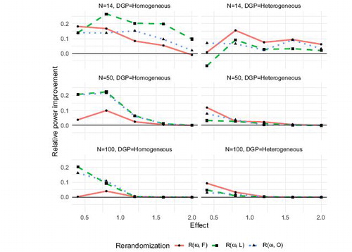
Fig. 6 Relative power as compared to complete randomization the ranked p-values (R) rerandomization designs with forecast-based and LASSO estimated weights, respectively, for T = 100. The left panel and right panel display the results from the homogenous and the heterogeneous DGP’s, respectively.

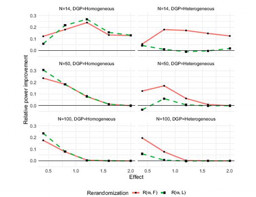
Table 4 Relative change in variance in the estimated treatment effect as compared to complete randomization (Equations (15)(15) $$\text{VC}(k|d)\equiv \frac{\text{var}({\overline{\mathbf{Z}}}_{kT}-{\overline{\mathbf{Z}}}_{kT}|d)-\text{var}({\overline{\mathbf{Z}}}_{kT}-{\overline{\mathbf{Z}}}_{kT}|c)}{\text{var}({\overline{\mathbf{Z}}}_{kT}-{\overline{\mathbf{Z}}}_{kT}|c)},$$(15) and (16)(16) $${\text{VC}}_{\tau }(d)\equiv \frac{\text{var}({\widehat{\tau }}_d)-\text{var}({\widehat{\tau }}_c)}{\text{var}({\widehat{\tau }}_c)}.$$(16) ) for the ranked p-values (R) rerandomization designs with forecast-based and LASSO estimated weights, respectively.

Rerandomization	$R(\omega ,F)$			$R(\omega ,L)$
N	14	50	100	14	50	100
	Homogeneous
VC τ(.)	–0.19	–0.25	–0.21	–0.22	–0.25	–0.24
	Heterogeneous
VC τ(.)	–0.23	–0.26	–0.22	–0.07	–0.11	–0.06

NOTE: The top and bottom panels display the results for the homogeneous and heterogeneous DGPs, respectively.

Fig. 7 The electricity consumption (kWh) for the households with the largest (max) and smallest (min) maximum consumption, mean consumption, and standard deviation in their consumption, respectively.

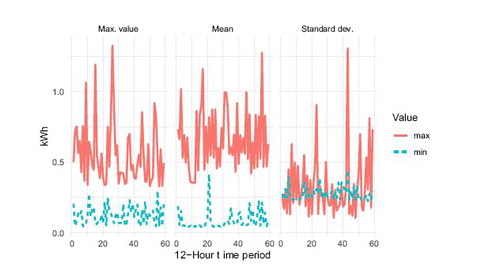
Fig. 8 The relative probability as compared to complete randomization of randomly selecting an allocation that gives a significant result for two different rerandomization strategies given different hypothesized treatment effects.

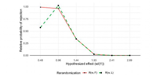
Table 5 Relative variance change in the effect estimates across the possible allocation using $R(\omega ,F)$ and $R(\omega ,L)$ as compared to complete randomization (Equation (16)(16) $${\text{VC}}_{\tau }(d)\equiv \frac{\text{var}({\widehat{\tau }}_d)-\text{var}({\widehat{\tau }}_c)}{\text{var}({\widehat{\tau }}_c)}.$$(16) ).

Rerandomization	$R(\omega ,F)$	$R(\omega ,L)$
VC τ(.)	–0.56	–0.61

NOTE: Complete randomization is here Monte Carlo approximated by 40,000 random allocations.