Local biplots for multidimensional scaling, with application to the microbiome

Figures & data

Fig. 1 Phylogenetic tree $\mathcal{T}$ (top) and simulated data $\mathbf{X}$ (bottom). White boxes indicate 0 abundance in the data matrix $\mathbf{X}$, and other colors from light to dark indicate low to high non-zero abundances. Samples are encoded in rows, and variables in the columns. Each variable corresponds to one tip of the tree, and the colored shapes at the tips of the tree represent the variables. The variable colors and shapes are carried through to Figure 3.

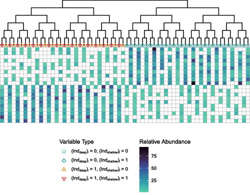
Fig. 2 Classical multidimensional scaling representation of the samples in the simulated dataset using the weighted UniFrac distance (left) and Manhattan distance (right). Each point represents a sample, and shape represents which group the sample came from.

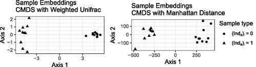
Fig. 3 Local biplot axes for CMDS/weighted UniFrac (top) and CMDS/Manhattan distance (bottom). One set of local biplot axes is plotted for each sample point. A segment connected to a sample point represents a local biplot axis for one variable at that sample point. The shape/color at the end of a local biplot axis represents variable type, and matches the shapes/colors of the points on the tips of the trees in Figure 1.

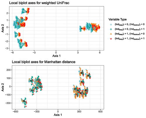
Fig. 4 Correlation biplot axes for weighted UniFrac (left) and Manhattan distance (right). Each segment is a biplot axis. The shape/color at the end of each biplot axis represents variable type, and matches the shape/color of the points on the tips of the trees in Figure 1.

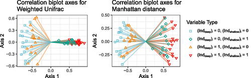
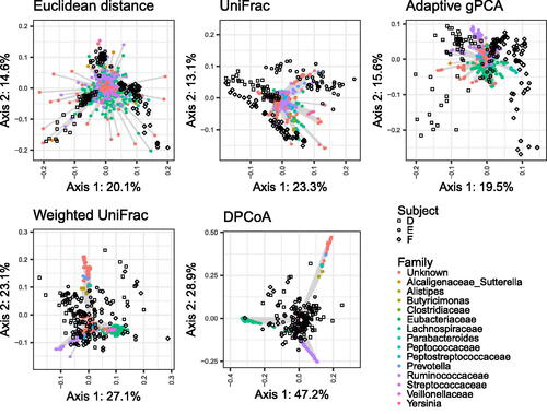
Fig. 5 Biplots for CMDS of the micobiome data with each of the five distances. Samples are shown as black shapes, and biplot axes are shown as colored circles connected to gray line sigments. Local biplot axes are shown for only one point to avoid cluttering the display. Biplot axis points are colored according to the family the taxon is associated with.