Linear Aggregation in Tree-Based Estimators

Figures & data

Fig. 1 Comparison of the classical CART and LRT. The top of the figure shows the fit of LRT and the fit of classical CART, and the lower part shows the density of the training set.

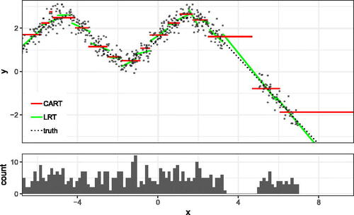
Table D1 Above displays the software packages and tuned hyperparameters used by the caret package for each estimator in Section 3.

Estimator	Package	Tuned Hyperparameters
Random Forest	ranger	mtry, min.node.size, num.trees, sample.fraction
Random Forest	Rforestry	mtry, nodesizeStrictSpl, ntree, sample.fraction
Linear Random Forest	Rforestry	mtry, nodesizeStrictSpl, ntree,
		sample.fraction, overfitPenalty, minSplitGain
Regularized Linear Model	glmnet	alpha, lambda
Cubist	Cubist	committees, extrapolation, neighbors
Bayesian Additive Regression Trees	dbarts	base, power, ntree, sigdf
Local Linear Forest	grf	mtry, min.node.size, num.trees, sample.fraction
Linear CART	Rforestry	mtry, nodesizeStrictSpl,
		overfitPenalty, minSplitGain

NOTE: For the exact hyperparameter values selected by the caret package, see the replication archive at https://github.com/forestry-labs/RidgePaperReplication

Fig. 2 Different levels of smoothness. In Experiment 1, the response surface is a linear function, in Experiment 2, it is a step function, and in Experiment 3, it is partly a step function and partly a linear function.

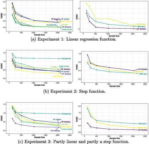
Table 1 Summary of real world datasets.

name	ntrain	ntest	dim	numeric features
Abalone	2089	2088	11	11
Autos	1206	39,001	12	6
Bike	869	16,510	16	16
Boston	506		9	9
Friedman 1	1000	2000	11	11
Friedman 2	1000	2000	5	5
Friedman 3	1000	2000	5	5
Ozone	330		9	9
Servo	167		13	13

Table 2 Estimator RMSE compared across real world datasets.

NOTE: The final row displays the mean performance rank across the different datasets for each estimator.

Fig. 3 The mean Ridge Coefficients from simulated data generated according to Equation (10)(10) $$Y=\varsigma \left(X_1\right)\varsigma \left(X_2\right)+\varsigma \left(X_3\right)\varsigma \left(X_4\right)+ϵ$$(10) , repeated over 100 Monte Carlo replications. The true outcome relies on only the first four covariates, and these coefficients have nonzero slope which is picked up by the LRF. The horizontal line corresponds to 1.96 times the sample standard deviation of the coefficients over the Monte Carlo replications.

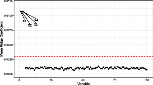
Fig. 4 The first tree of the S-Learner as described in Section 4.2. The first row in each leaf contains the number of observations in the averaging set that fall into the leaf. The second part of each leaf displays the regression coefficients. Baseline stands for untreated base turnout of that leaf and it can be interpreted as the proportion of units that fall into that leaf who voted in the 2004 general election. Each coefficient corresponds to the ATE of the specific mailer in the leaf. The color strength is chosen proportional to the treatment effect for the neighbors treatment.

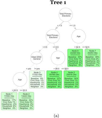
Fig. A1 This example has a piecewise linear response, with alternating slopes in the first covariate. Here we plot X₁ against the outcome y, and overlay the fitted values which are returned by both the Local Linear Forest and Linear Regression Tree.

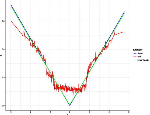
Fig. H1 The next three trees of the S-Learner as described in Section 4.2. The first row in each leaf contains the number of observations in the averaging set that fall into the leaf. The second part of each leaf displays the regression coefficients. Baseline stands for untreated base turnout of that leaf and it can be interpreted as the proportion of units that fall into that leaf who voted in the 2004 general election. Each coefficient corresponds to the ATE of the specific mailer in the leaf. The color strength is chosen proportional to the treatment effect for the neighbors treatment.

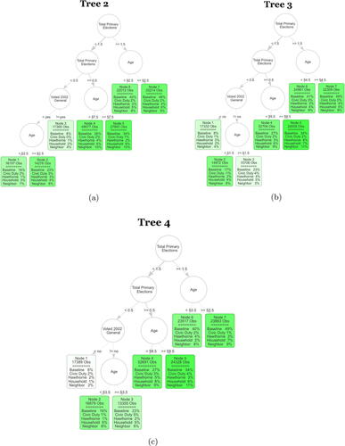
Fig. I1 The left shows the mean normalized variable importances from LRF on simulated data, repeated over 100 Monte Carlo replications. The right shows the mean normalized variable importances from RF on simulated data, repeated over 100 Monte Carlo replications. The true outcome relies on only the first four covariates.

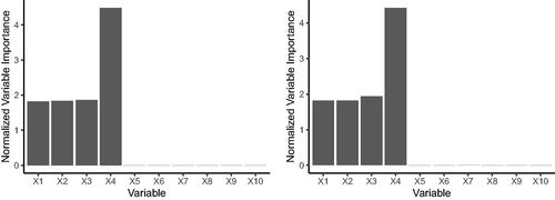
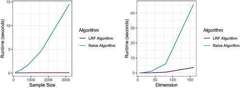
Fig. J1 We run both the naive linear regression tree algorithm and the fast LRF algorithm from Section 2 for 100 Monte Carlo replications on the same data generated according to Equation 25(25) $$Y=.4X_1+2X_2-.9X_3+.25X_4+ϵ$$(25) . The left figure shows the mean timing of both algorithms as we keep the dimension fixed and vary the sample size, and the right figure shows the mean timing of both algorithms as we fix the sample size and vary the dimension.

Data Availability Statement

Code for replication of results can be found at https://github.com/forestry-labs/RidgePaperReplication.

The Rforestry package can be found at https://github.com/forestry-labs/Rforestry