Connecting the Dots: Numerical Randomized Hamiltonian Monte Carlo with State-Dependent Event Rates

Figures & data

Fig. 1 Empirical cumulative distribution functions (CDFs) associated with MCMC output for the standard Gaussian ${\mathit{q}}_1$-marginal under the “funnel”-model ${\mathit{q}}_1\sim N(0,1)$, ${\mathit{q}}_2|{\mathit{q}}_1\sim N(0,\hspace{0.17em}\text{exp}\hspace{0.17em}(3{\mathit{q}}_1))$. For visual clarity, only the left half of the distributions are presented. Further details on this experiment can be found in Section 5.1. Each case is based on 5000 samples from each of 10 independent replica. The black solid lines are the empirical CDFs, whereas the red dashed lines are the true CDFs. The shaded gray region would cover 90% of empirical CDFs based on 50,000 iid N(0, 1) samples point-wise. The four left-most panels are based on Stan output with different values of the accept rate target δ. In practice, higher values of δ corresponds to smaller integrator step sizes and more integrator steps per produced sample. The right-most panel shows output for the proposed methodology using constant event rates. For both Stan and the proposed methodology, an identity mass matrix was employed.

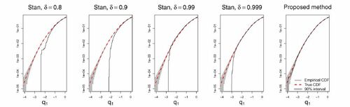
Table 1 The event specifications applied in the reminder of this text.

Event specification	λ	$K_{\mathit{q}}(\mathit{p}|{\mathit{p}}^{\prime })$	Interpretation
1	$\frac{1}{\beta }$	$\mathcal{N}\left(\mathit{p}\right|\varphi {\mathit{p}}^{\prime },\sqrt{1-{\varphi }^2}\mathit{M}),\varphi \in (-1,1)$	Time between events is $\text{Exp}\hspace{0.17em}(\beta$), autocorrelated momentum refreshes
2	$\frac{1}{\beta }\sqrt{{\mathit{p}}^T{\mathit{M}}^{-1}\mathit{p}}$	$\propto \sqrt{{\mathit{p}}^T{\mathit{M}}^{-1}\mathit{p}}\hspace{0.17em}\text{exp}\hspace{0.17em}\left(-\frac{1}{2}{\mathit{p}}^T{\mathit{M}}^{-1}\mathit{p}\right)\sim \sqrt{\frac{r}{{\mathit{y}}^T\mathit{y}}}\sqrt{\mathit{M}}\mathit{y},$ where $\mathit{y}\sim N({\mathbf{0}}_d,{\mathit{I}}_d),r\sim {\chi }^2(d+1)$	Arc-length of between-events (standardized) position trajectory is $\text{Exp}\hspace{0.17em}(\beta )$, independent momentum refreshes

NOTE: In all cases β is a tuning parameter, where larger βs on average correspond to less frequent events/longer inter-event trajectories. For specification 2, arc-lengths of position-trajectories are calculated in the Mahalanobis distance $d(\mathit{q},{\mathit{q}}^{\prime })=\sqrt{{(\mathit{q}-{\mathit{q}}^{\prime })}^T\mathit{M}(\mathit{q}-{\mathit{q}}^{\prime })}$ as ${\mathit{M}}^{-1}$ is assumed to be some approximation/reflect the scales of the covariance matrix of $\pi (\mathit{q})$.

Fig. 2 Examples of q-coordinate of continuous time HMC trajectories with different event specifications for a bivariate standard Gaussian target distribution $\pi (\mathit{q})$. In all cases, $\mathit{M}={\mathit{I}}_2$ and the shown trajectories correspond 100 units of time t. Events are indicated with red circles, and the common initial q-coordinate is indicated with a cross. In the rightmost panel, an event rate favoring events when the distance between the q-coordinate and its projection onto the subspace spanned by $\mathit{v}=(1,1)$ (indicated by a gray line) is small.

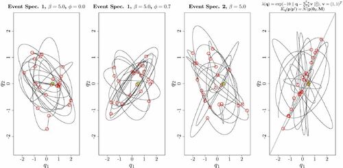
Fig. 3 RMSE of estimates of $E({\mathit{q}}_1)$ from NGRHMC processes using event specification 1 for different values of the mean inter-event time parameter β. The panels correspond to the different univariate target distributions $\pi ({\mathit{q}}_1)$, which all have zero mean and unit variance. Unit mass matrix M = 1 was used. The estimates of the mean are based on trajectories of length $T=1000\frac{\pi }{2}$, and the RMSE estimates are based on 10,000 independent replica for each value of β. Black circles correspond continuous sampling (7), red ×-s to 1000 equally spaced samples, blue squares to 500 equally spaced samples and green triangles to samples recorded at events only. The horizontal lines give the RMSE of 1000 iid samples. The results are obtained using the numerical methods described in Section 4.1 with $to{l}_a=to{l}_r=0.001$.

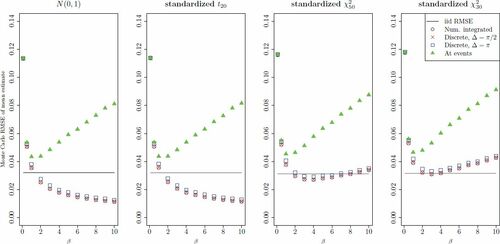
Table 2 Results for the “smile”-shaped target distribution (22,23).

γ	sampling		${\mathit{q}}_1$		$\underset{k\in \{2,11\}}{\min }\text{ESS}({\mathit{q}}_k)$		$\underset{k\in \{2,11\}}{\max }\text{ESS}({\mathit{q}}_k)$		$E({\mathit{q}}_1)$	$E({\mathit{q}}_2)$	CPU time
			ESS	$\frac{\text{ESS}}{\text{CPU}\mathrm{}\text{time}}$	ESS	$\frac{\text{ESS}}{\text{CPU}\mathrm{}\text{time}}$	ESS	$\frac{\text{ESS}}{\text{CPU}\mathrm{}\text{time}}$	(exact $=0$)	(exact $=1$)	(s)
rstan ($\max \widehat{R}=1.247$)
			19	10	29	15	32	17	–0.15	1.04	1.9
pdphmc, event specification 1, $\varphi =0$ (γ = 2: $\max \widehat{R}=1.006$, γ = 10: $\max \widehat{R}=1.015$)
2	D		1323	779	1065	627	1215	716	–0.02	1.03	1.7
2	C		1319	777	1115	657	1150	678	–0.02	1.02
10	D		2213	1304	608	358	634	374	0.01	1.00	1.7
10	C		2233	1316	613	361	630	371	0.01	1.01
pdphmc, event specification 2 (γ = 2: $\max \widehat{R}=1.007$, γ = 10: $\max \widehat{R}=1.009$)
2		D	1094	645	1130	666	1183	697	–0.02	0.98	1.7
2		C	1094	645	1153	679	1184	698	–0.02	0.97
10		D	2276	1341	920	542	967	570	0.01	1.03	1.7
10		C	2303	1357	927	546	948	559	0.01	1.03

NOTE: The results are based on 10 independent replica, and ESSes and ESSes per computing time are from the combined results over these replica. For rstan, each replica consists of the 10,000 transitions, with the former 5000 discarded as warmup. For pdphmc, ISG-type mass matrix, trajectories of length T = 25,000 divided evenly between warmup and sampling, and 1000 discrete samples were used. The presented CPU times are the total time spent by all chains/trajectories during the post warmup period. For each configuration of pdphmc, results from both discrete sampling (D) and continuous sampling (C) are presented.

Fig. 4 Numerical errors incurred by RKN integration on the estimation the first and second order moments of a bivariate Gaussian target distribution. The numerical errors are relative to a NGRHMC trajectory using the same random numbers but with exact Hamiltonian dynamics. Both exact and numerically integrated results are based on continuous sampling. The horizontal axis gives the error tolerances (in all cases with $to{l}_a=to{l}_r$) applied in the numerical integrator, and both horizontal and vertical axis are logarithmic. Dotted lines indicate the root mean squared errors associated with estimating the indicated moments across many exact NGRHMC trajectories of different length T.

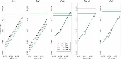
Table 3 ESSes and time weighted ESSes for the logistic regression model (24,25) applied to the German credit data.

γ	Sampling	${\min }_j$ $\widehat{\text{ESS}}({\mathit{\beta }}_j)$		${\text{median}}_j$ $\widehat{\text{ESS}}({\mathit{\beta }}_j)$		${\max }_j$ $\widehat{\text{ESS}}({\mathit{\beta }}_j)$		CPU
		ESS	$\frac{\text{ESS}}{\text{CPU}\mathrm{}\text{time}}$	ESS	$\frac{\text{ESS}}{\text{CPU}\mathrm{}\text{time}}$	ESS	$\frac{\text{ESS}}{\text{CPU}\mathrm{}\text{time}}$	time
rstan ($\max \widehat{R}=1.003$)
		9676	2125	13450	2953	15812	3472	4.55
pdphmc, event specification 1 (γ = 5: $\max \widehat{R}=1.011$, γ = 20: $\max \widehat{R}=1.020$)
5	D	11350	1425	23114	2903	40000	5023	7.96
5	C	18220	2288	32967	4140	71079	8926
20	D	11853	1490	29752	3740	40000	5028	7.96
20	C	20423	2567	36019	4528	69623	8752
pdphmc, event specification 2 ($\gamma =5$: $\max \widehat{R}=1.007$, γ = 20: $\max \widehat{R}=1.027$)
5	D	11281	1362	23185	2799	40000	4829	8.28
5	C	18317	2211	30771	3715	66928	8080
20	D	12780	1565	32653	3999	40000	4899	8.16
20	C	20902	2560	43303	5304	70584	8645

NOTE: All figures are based on 10 independent chains/trajectories. For rstan, the default 1000 warmup transitions followed by 1000 sampling transitions were used. For pdphmc, a VARI mass matrix, T = 5000 divided evenly between warmup and sampling and 1000 discrete samples per trajectory were used.

Table 4 Effective sample sizes and computing times for the dynamic inverted Wishart model (26,29).

		rstan	pdphmc, event spec. 1, $\gamma =10.0$ (10629, 25244) 1.032		pdphmc, event spec. 2, $\gamma =10.0$ (10189, 24960) 1.034
	CPU time (S,A)	(14605, 72127)
	$\max \widehat{R}$	1.003
	sampling		D	C	D	C
$\mathit{\mu }$	ESS (min, max)	(14304, 18487)	(12906, 28173)	(14467, 28370)	(14749, 38387)	(14224, 41821)
	ESS/S (min, max)	(0.98, 1.27)	(1.21, 2.65)	(1.36, 2.67)	(1.45, 3.77)	(1.40, 4.10)
	ESS/A (min, max)	(0.20, 0.26)	(0.51, 1.12)	(0.57, 1.12)	(0.59, 1.54)	(0.57, 1.68)
$\mathit{\sigma }$	ESS (min, max)	(14757, 20011)	(28447, 38922)	(35971, 42891)	(30227, 40000)	(34283, 44316)
	ESS/S (min, max)	(1.01, 1.37)	(2.68, 3.66)	(3.38, 4.04)	(2.97, 3.93)	(3.36, 4.35)
	ESS/A (min, max)	(0.20, 0.28)	(1.13, 1.54)	(1.42, 1.70)	(1.21, 1.60)	(1.37, 1.78)
$\mathit{\delta }$	ESS (min, max)	(13624, 16678)	(16145, 28401)	(18109, 31180)	(15749, 25582)	(9464, 29271)
	ESS/S (min, max)	(0.93, 1.14)	(1.52, 2.67)	(1.70, 2.93)	(1.55, 2.51)	(0.93, 2.87)
	ESS/A (min, max)	(0.19, 0.23)	(0.64, 1.13)	(0.72, 1.24)	(0.63, 1.02)	(0.38, 1.17)
H	ESS (min, max)	(12195, 22072)	(35292, 40000)	(46273, 69861)	(33089, 40000)	(43658, 70275)
	ESS/S (min, max)	(0.84, 1.51)	(3.32, 3.76)	(4.35, 6.57)	(3.25, 3.93)	(4.28, 6.90)
	ESS/A (min, max)	(0.17, 0.31)	(1.40, 1.58)	(1.83, 2.77)	(1.33, 1.60)	(1.75, 2.82)
ν	ESS	17797	40000	53388	40000	56313
	ESS/S	1.22	3.76	5.02	3.93	5.53
	ESS/A	0.25	1.58	2.11	1.60	2.26
${\mathit{z}}_{1,·}$	ESS (min, max)	(22130, 24317)	(30533, 40000)	(37065, 70920)	(40000, 40000)	(64787, 68952)
	ESS/S (min, max)	(1.52, 1.67)	(2.87, 3.76)	(3.49, 6.67)	(3.93, 3.93)	(6.36, 6.77)
	ESS/A (min, max)	(0.31, 0.34)	(1.21, 1.58)	(1.47, 2.81)	(1.60, 1.60)	(2.60, 2.76)
${\mathit{x}}_{1,·}$	ESS (min, max)	(22149, 24858)	(27525, 40000)	(33768, 70763)	(40000, 40000)	(63230, 68873)
	ESS/S (min, max)	(1.52, 1.70)	(2.59, 3.76)	(3.18, 6.66)	(3.93, 3.93)	(6.21, 6.76)
	ESS/A (min, max)	(0.31, 0.34)	(1.09, 1.58)	(1.34, 2.80)	(1.60, 1.60)	(2.53, 2.76)

NOTE: In all cases, the results are based on 10 independent chains/trajectories and reported computing times are the total computing times over these 10 replica. For rstan, default sampler parameters with 1000 warmup transitions followed by 1000 sampling transitions were used. For pdphmc, T = 5000 split evenly between warmup and sampling, 1000 samples and an VARI type diagonal mass matrix were applied. Both computing times for the sampling (S) period and for all (A) computations (warmup and sampling) are provided, and ESSes are weighted both for S and A.