Statistical Analysis of Locally Parameterized Shapes

Figures & data

Fig. 1 Problem of false positives due to alignment. (a) Two ellipsoidals are depicted by line and dashed line. Circles and crosses show corresponding boundary points. Bold points are shapes’ centroids. (b) Two populations of simulated PDMs. (c), (d), (e) Separation of corresponding local distributions.

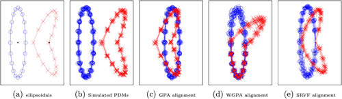
Fig. 2 Skeletal structure of ellipsoidal objects. (a) 2D m-reps. s and $\mathit{s}\prime$ are corresponding spokes with unit directions u and $\mathit{u}\prime$. (b) A fitted ds-rep to a left hippocampus’s mesh including up, down, crest spokes, and the skeletal sheet.

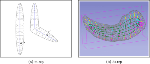
Fig. 3 (a) Illustration of a 2D-ellipsoidal (left) approximated by a perfect 2D-ellipsoidal (right). The solid curve and the bold dot (right) depict the medial curve and medial centroid, respectively. (b) Left: A mandible (without coronoid processes) as an example of a 3D-ellipsoidal with slicing planes. The solid curve is the center curve. Right: A cross-section as a 2D-ellipsoidal including its medial curve.

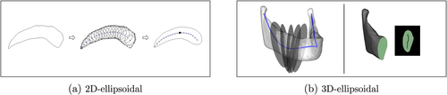
Fig. 4 Skeletal sheet. Left: Ellipsoid’s medial locus. Right: s-rep skeletal sheet of a 3D-ellipsoidal.

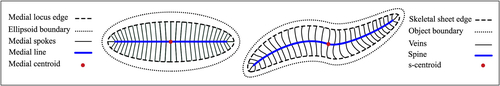
Fig. 5 Illustration of a local frame. n is normal to tangent planes $T_{\mathit{p}}(M)$ and $T_{\mathit{p}}(M_{\Omega })$. (a) ${\mathit{s}}_1$ and ${\mathit{s}}_2$ are equal-length spokes with unit directions ${\mathit{u}}_1$ and ${\mathit{u}}_2$, and $\mathit{b}=\frac{{\mathit{u}}_1+{\mathit{u}}_2}{\left|\right|{\mathit{u}}_1+{\mathit{u}}_2\left|\right|}$ (b) c is a smooth curve on M. $-\mathit{p}{\prime }_1$ and $\mathit{p}{\prime }_2$ are the projection of ${\mathit{p}}_1$ and ${\mathit{p}}_2$ on $T_{\mathit{p}}(M)$. $\widehat{\mathit{v}}{\prime }_1=\frac{\mathit{p}-\mathit{p}{\prime }_1}{\left|\right|\mathit{p}-\mathit{p}{\prime }_1\left|\right|}$, $\widehat{\mathit{v}}{\prime }_2=\frac{\mathit{p}{\prime }_2-\mathit{p}}{\left|\right|\mathit{p}{\prime }_2-\mathit{p}\left|\right|}$, and $\mathit{b}=\frac{\widehat{\mathit{v}}{\prime }_2+\widehat{\mathit{v}}{\prime }_1}{\left|\right|\widehat{\mathit{v}}{\prime }_2+\widehat{\mathit{v}}{\prime }_1\left|\right|}$.

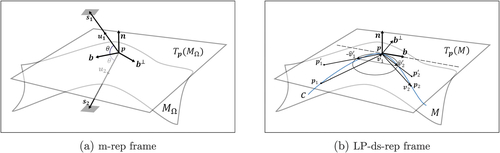
Fig. 6 LP-ds-rep. Top: Hierarchical structure of the ellipsoid’s medial locus. Arrows are connections. The dot is the medial centroid. Bottom: A fitted LP-ds-rep to a hippocampus. Arrows indicate spokes, connections, and frames. The magnified image depicts a spinal frame. The dot is the s-centroid.

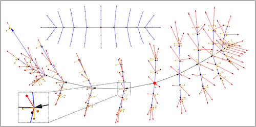
Fig. 7 Skeletal deformation by LP-ds-rep. Left: A ds-rep with its implied boundary in two angles. Middle: Shape bending by spinal frame rotation about n and ${\mathit{b}}^{\perp }$ axes. Right: Shape twisting by spinal frames rotation about b axis.

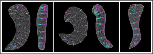
Fig. 8 Simulation. Left: Two groups of simulated ds-reps. Middle: Overlaid mean LP-ds-reps. Right: Illustration of local frames. Bold frames are statistically significant.

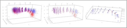
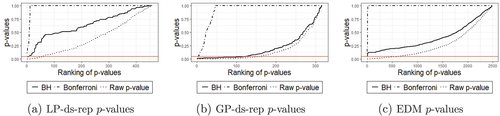
Fig. 9 Sorted raw and adjusted p-values. The horizontal line indicates significance level $\alpha =0.05$.

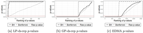
Table 1 T-test on shape size.

	Mean CG	Mean PD	SD CG	SD PD	p-value
Object volume (mm^3)	3352.23	3271.44	563.39	616.68	0.26
LP-size	2.37	2.33	0.17	0.18	0.04
GP-size of spokes’ tips	161.05	162.51	8.97	8.62	0.17
EDM-size of skeletal PDM	12.66	12.76	0.83	0.84	0.36

Fig. 10 ds-rep significant GOPs. Bold indicate significant GOPs. FDR = 0.05 for BH adjustment.

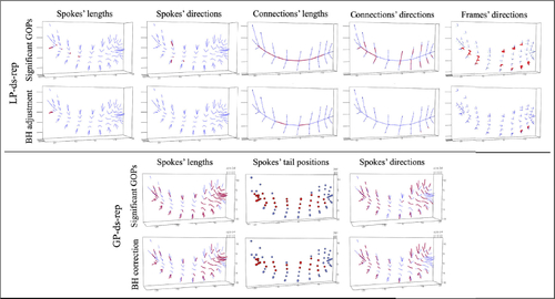
Fig. 11 Test on real data. Sorted raw and adjusted p-values. The horizontal line indicates significance level 0.05.