Fast, Approximate Maximum Likelihood Estimation of Log-Gaussian Cox Processes

Figures & data

Fig. 1 A: An observed point pattern of gorilla nesting locations in Kagwene Gorilla Sanctuary in Cameroon. B: An inhomogeneous K function for the point pattern (Baddeley and Turner 2000), with simulation envelope (computed as in Myllymäki et al. 2017), to check goodness of fit under an IPP model (top panel) and LGCP model (bottom panel). For model details see Section 5. Note there is evidence of additional spatial clustering to that accounted for by the IPP model, but not so for the LGCP.

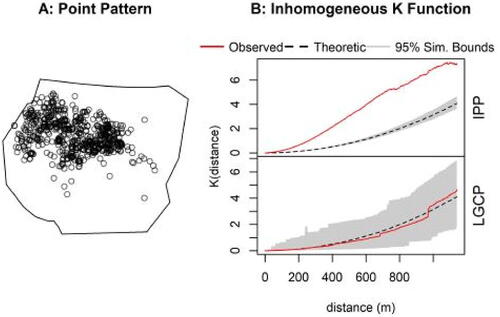
Fig. 2 The 2 × 2 simulation design showing the scenarios examined. Deterministic functions are used for the covariate ($X(\mathit{s})$) while particular examples of the latent field, $\xi (\mathit{s})$, are shown here. “Smooth” means a range of effect $\approx 0.3$ while “wiggly” means a range of effect $\approx 0.05$, with the spatial domain being the unit square.

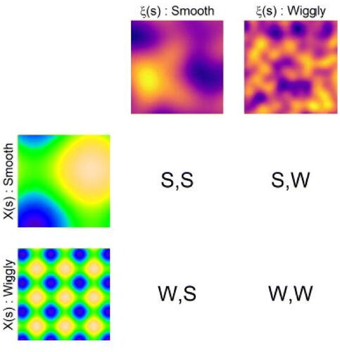
Fig. 3 Average computation times over variously sized point patterns ($\mathbb{E}\left[N(\mathcal{D})\right]=1 000,10,000,100,000$)—see supplementary material: Section S2.2 for details. Models include IPP, INLA, spNNGP and our proposed method using variational (VA) and Laplace (Lp) approximations. The latter two models were fitted both using a coarse regular grid of basis functions, 7 × 7 and a fine regular grid, 14 × 14. For small point patterns our methods were at least 50 times faster than INLA on average. For large point patterns they were as much as 1000 times faster than INLA on average.

Fig. 4 Performance of point and interval estimators for the various models, across simulation scenarios using either a wiggly (W) or a smooth (S) covariate and latent field (labeled with the covariate first, for example, “W,S” means the covariate is wiggly and the latent field smooth). A: Root mean squared error estimating the slope coefficient β₁. B: Kullback-Leibler divergence from the true intensity field $\lambda (\mathcal{D})$ to that fitted by each model. C: Coverage probabilities of 95% Wald intervals for the slope estimate, $\widehat{{\beta }_1}$ (dotted vertical line indicates nominal coverage). We found that, provided we choose the most appropriate basis function configuration for the scenario, our proposed methods performed comparably to INLA in point estimation of β₁, and for Lp, also in estimation of intensity and interval coverage.

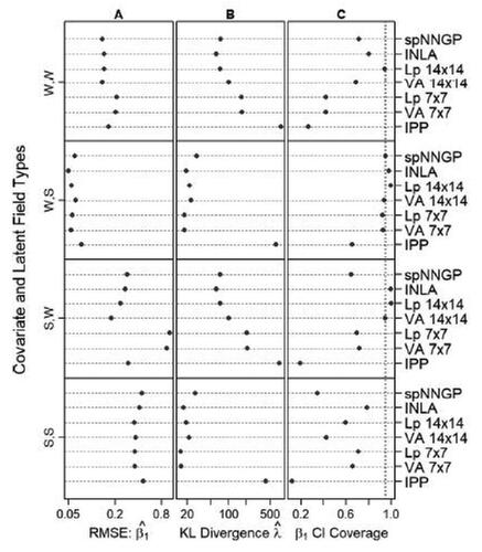
Table 1 Four-fold cross-validated predicted conditional log-likelihoods of the various models and corresponding computation times.

	INLA	LP	VA	IPP
Predicted $\mathcal{l}(\mathit{\beta }|\mathit{\xi })$	2307.7	2299.8	2301.4	1727.5
Comp. Time	46.79 min	31.88 sec	13.17 sec	0.67 sec

NOTE: We see that our proposed methods (LP and VA) achieved comparable predicted conditional log-likelihoods, in under a minute, compared to INLA that took over 45 min.

Fig. 5 A: Spatial covariate describing elevation in meters above sea level. B: Spatial covariate describing distance in meters to nearest water source. C: Factor describing heat category: 1 = Coolest, 2 = Moderate, 3 = Warmest. D: Latent field (conditional on the data) estimated by VA method. E: Latent field (conditional on the data) estimated by INLA. F: Spatially blocked four-fold cross-validation.

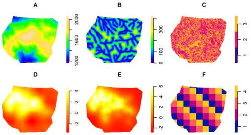
Fig. 6 The variational approximation to the marginal log-likelihood of the proposed LGCP model as a function of increasingly dense regular grids of local bi-square basis functions. The vertical dashed line denotes the basis functions at which the maximum is found. Secondary plot and axis (gray) indicates the cumulative computational time, in seconds, taken to fit models using each of the basis function configurations.

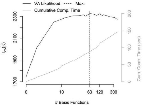
Table 2 The computation time and likelihood for a single model fit for our proposed model for which we toggled on/off key components—a variational approximation for the marginalization (VA, vs. Laplace approximation, Lp); automatic differentiation (AD); sparse basis approximation for the latent field (Sparse/Dense Z); and large number of basis functions (Large k).

Method	Sparse/dense Z	AD	Large k	Comp. Time (sec)	$\mathcal{l}(\mathit{\beta })$
VA	Sparse	✓		4.30	2323.78
Lp	Sparse	✓		16.10	2333.62
VA	Dense	✓		41.80	2271.96
VA	Sparse			93.60	2323.78
VA	Sparse	✓	✓	96.19	2187.01
INLA			✓	718.87	2336.70

NOTE: INLA is also included for comparison.

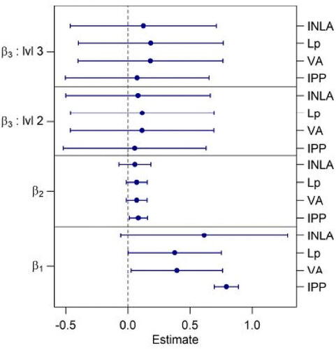
Fig. 7 Estimated fixed effects 95% Wald confidence intervals for the various models being compared. (a) Elevation effect. (b) Distance to water effect. (c) Heat category—contrast effect of Moderate to Coolest. (d) Heat category—contrast effect of Warmest to Coolest. We see little difference in the estimated fixed effects for the LGCP models (INLA, VA, Lp), so much of the differences in predictive performance came down to the way the latent effect was modeled (or was not modeled for the IPP).

Baddeley, A., and Turner, R. (2000), “Practical Maximum Pseudolikelihood for Spatial Point Patterns” (with discussion), Australian & New Zealand Journal of Statistics, 42, 283–322. DOI: 10.1111/1467-842X.00128.

 Web of Science ®Google Scholar

Myllymäki, M., Mrkvicka, T., Grabarnik, P., Seijo, H., and Hahn, U. (2017), “Global Envelope Tests for Spatial Processes,” Journal of the Royal Statistical Society, Series B, 79, 381–404. DOI: 10.1111/rssb.12172.

 Google Scholar