Local Inhomogeneous Weighted Summary Statistics for Marked Point Processes

Figures & data

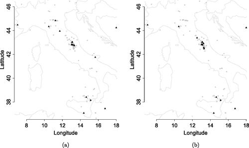
Fig. 1 The Italian seismic dataset for machine learning (INSTANCE). (a) Earthquake locations; (b) Seismic stations used for waveforms extraction. The symbol sizes are proportional to earthquake magnitude and number of arrival phases recorded by stations, respectively; (c) Seismic waveforms of some events with magnitude in the range $[2,4]$. Vertical lines indicate the seismic waves’ arrival times. Source: Michelini et al. (2021).

Fig. 2 (a) Simulated earthquake locations. (b) Simulated waveform marking the highlighted point on panel (a). (c) Result of the global test.

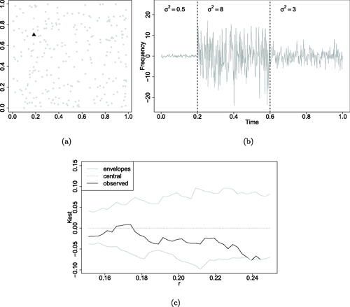
Fig. 3 (a) Result of global test for the spatially dependent simulated data. (b) Output of the local test: the black triangles are the significant points for which the hypothesis of random labeling is rejected.

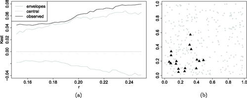
Fig. 4 Simulation scenarios. (a)–(c) Spatial ground patterns; (d)–(f) Functional marks of model (11) (in gray) and of the marking models in item 1, 2, and 3, respectively (in black).

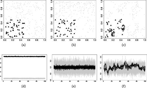
Table 1 Results of the local test averaged over 100 simulated point patterns with an expected point count of 250 each.

Ground process	Marking model	TPR	FPR	ACC
Homogeneous Poisson	(1)	0.112	0.346	0.583
Homogeneous Poisson	(2)	0.583	0.066	0.820
Homogeneous Poisson	(3)	0.870	0.024	0.896
Inhomogeneous Poisson	(1)	0.032	0.585	0.449
Inhomogeneous Poisson	(2)	0.648	0.084	0.856
Inhomogeneous Poisson	(3)	0.895	0.023	0.932
Thomas	(1)	0.109	0.394	0.571
Thomas	(2)	0.637	0.088	0.846
Thomas	(3)	0.865	0.025	0.925

Fig. 5 Earthquake locations.

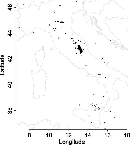
Fig. 6 Local K-functions. (a) The K-function is based on a kernel intensity estimate whose bandwidth is selected by Diggle’s (2013) rule. (b) The bandwidth is chosen as in Cronie and Van Lieshout (2018).

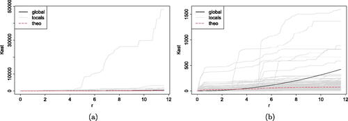
Fig. 7 Results of the local test at $\alpha =0.1$. Nonsignificant events are displayed as gray points and significant events are the black triangles. (a) The K-function is based on a kernel intensity estimate whose bandwidth is selected by Diggle’s (2013) rule. (b) The bandwidth is chosen as in Cronie and Van Lieshout (2018).

Michelini, A., Cianetti, S., Gaviano, S., Giunchi, C., Jozinović, D., and Lauciani, V. (2021), “Instance–The Italian Seismic Dataset for Machine Learning,” Earth System Science Data, 13, 5509–5544. DOI: 10.5194/essd-13-5509-2021.

 Web of Science ®Google Scholar

Diggle, P. (2013), Statistical Analysis of Spatial and Spatio-Temporal Point Patterns. Boca Raton, FL: CRC Press.

 Google Scholar

Cronie, O., and van Lieshout, M. N. M. (2018), “A Non-Model-based Approach to Bandwidth Selection for Kernel Estimators of Spatial Intensity Functions,” Biometrika, 105, 455–462.

 Web of Science ®Google Scholar