Convolutional Neural Networks for Valid and Efficient Causal Inference

Figures & data

Fig. 1 Illustration of the convolutional neural network used in the simulations and the real data study. Each layer, $i\in \{0,\dots ,l\}$ contains different number of channels E_i, where E₀ (not shown in the figure) is the number of time series in the set of input covariates. Each channel (feature map) in a given layer is formed by first applying $E_{i-1}$ number of kernels (convolution filters) on the vectors in layer i–1 and then summing the results. There exist some covariates which are not time series. Inclusion of those vectors in the neural network is not illustrated in the figure for simplification purpose. A fully connected feed-forward structure has been used for those covariates and the results are then combined with the results from the time-series data in the flattening layer demonstrated above.

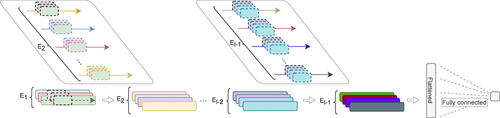
Table 1 Setting 1 DGP: Bias, standard errors (both estimated, Est sd, and Monte Carlo, MC sd), MSEs and empirical coverages for 95% confidence intervals over 1000 replicates.

	bias	coverage	MC sd	Est sd	MSE
n = 5000
DRcnn	0.185	0.947	1.379	1.366	1.935
DRmlp	0.426	0.940	1.353	1.331	2.013
ORds	0.001	0.947	1.404	1.392	1.970
DRss	0.002	0.948	1.404	1.395	1.971
DRds	0.003	0.948	1.404	1.395	1.972
tmle	0.044	0.944	1.396	1.384	1.951
n = 10, 000
DRcnn	0.089	0.958	0.971	0.972	0.951
DRmlp	0.223	0.949	0.961	0.958	0.973
ORds	0.001	0.955	0.981	0.982	0.962
DRss	0.001	0.955	0.981	0.984	0.962
DRds	0.001	0.955	0.981	0.984	0.962
tmle	0.028	0.957	0.981	0.978	0.963

Table 2 Setting 2 DGP: Bias, standard errors (both estimated and Monte Carlo), MSEs and empirical coverages for 95% confidence intervals over 1000 replicates.

	bias	coverage	MC sd	Est sd	MSE
n = 5000
DRcnn	0.047	0.937	0.094	0.101	0.011
DRmlp	0.076	0.890	0.095	0.099	0.015
ORds	0.233	0.206	0.083	0.085	0.061
DRss	0.233	0.260	0.083	0.092	0.061
DRds	0.235	0.250	0.083	0.092	0.062
tmle	0.233	0.204	0.083	0.085	0.061
n = 10, 000
DRcnn	0.025	0.945	0.070	0.072	0.006
DRmlp	0.036	0.928	0.070	0.072	0.006
ORds	0.224	0.040	0.062	0.061	0.054
DRss	0.224	0.054	0.062	0.065	0.054
DRds	0.226	0.045	0.061	0.065	0.055
tmle	0.224	0.041	0.062	0.061	0.054

Fig. 2 Retirement age for men and women who belong to the cohorts born in Sweden 1946 and 1947. The last staple in each histogram displays those who retired at age 71 or later.

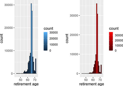
Table 4 Effect of early retirement on survival (binary outcomes death = 1), during five years of follow up for the early retirees, and 95% confidence intervals.

	Women n = 106,916		Men n = 105,149
The first year after treatment is considered for the outcome
naive	0.002		–0.001
DRcnn	0.005	(0.002, 0.008)	–0.001	(–0.005, 0.003)
DRmlp	0.004	(0.000, 0.007)	–0.003	(–0.013, 0.007)
ORds	0.003	(–0.194, 0.200)	0.000	(–0.150, 0.151)
DRss	0.003	(0.000, 0.006)	0.000	(–0.002, 0.003)
DRds	0.003	(0.000, 0.007)	0.000	(–0.002, 0.003)
tmle	0.003	(0.000, 0.006)	0.000	(–0.002, 0.003)
The second year after treatment is considered for the outcome
naive	0.002		–0.002
DRcnn	0.007	(0.003, 0.012)	0.001	(–0.005, 0.007)
DRmlp	0.006	(0.002, 0.011)	0.001	(–0.003, 0.006)
ORds	0.005	(–0.164, 0.174)	0.002	(–0.130, 0.133)
DRss	0.005	(0.001, 0.009)	0.002	(–0.002, 0.005)
DRds	0.005	(0.001, 0.009)	0.002	(–0.002, 0.005)
tmle	0.005	(0.001, 0.009)	0.002	(–0.002, 0.005)
The third year after treatment is considered for the outcome
naive	0.000		–0.002
DRcnn	–0.052	(–0.166, 0.063)	0.005	(0.000, 0.010)
DRmlp	0.004	(–0.001, 0.009)	0.008	(0.003, 0.013)
ORds	0.004	(–0.150, 0.159)	0.004	(–0.114, 0.122)
DRss	0.005	(0.000, 0.009)	0.004	(–0.000, 0.009)
DRds	0.005	(0.001, 0.010)	0.005	(0.000, 0.009)
tmle	0.005	(0.000, 0.009)	0.004	(–0.000, 0.009)
The fourth year after treatment is considered for the outcome
naive	–0.003		& -0.006
DRcnn	0.002	(–0.005, 0.008)	–0.001	(–0.007, 0.005)
DRmlp	0.001	(–0.005, 0.006)	0.005	(–0.000, 0.011)
ORds	0.003	(–0.140, 0.145)	0.002	(–0.107, 0.110)
DRss	0.003	(–0.002, 0.008)	0.002	(–0.003, 0.007)
DRds	0.004	(–0.001, 0.009)	0.002	(–0.003, 0.007)
tmle	0.003	(–0.002, 0.008)	0.002	(–0.003, 0.007)
The fifth year after treatment is considered for the outcome
naive	–0.005		–0.007
DRcnn	0.002	(–0.004, 0.009)	0.001	(–0.006, 0.008)
DRmlp	0.009	(0.002, 0.016)	0.009	(0.002, 0.016)
ORds	0.001	(–0.131, 0.134)	0.002	(–0.098, 0.102)
DRss	0.002	(–0.004, 0.008)	0.002	(–0.003, 0.008)
DRds	0.003	(–0.003, 0.008)	0.003	(–0.003, 0.009)
tmle	0.002	(–0.004, 0.008)	0.002	(–0.003, 0.008)

Table 3 Effect of early retirement on number of days in hospital during five years of follow up, for the early retirees, and 95% confidence intervals.

	Women		Men
The first year	n = 106,437		n = 104,459
naive	–0.396		–0.167
DRcnn	0.062	(–0.060, 0.183)	–0.037	(–0.256, 0.183)
DRmlp	–0.062	(–0.192, 0.069)	0.138	(–0.079, 0.355)
ORds	–0.135	(–0.231, –0.039)	0.018	(–0.156, 0.192)
DRss	–0.138	(–0.232, –0.045)	0.025	(–0.148, 0.199)
DRds	–0.128	(–0.222, –0.035)	0.028	(–0.145, 0.202)
tmle	–0.143	(–0.237, –0.049)	0.018	(–0.156, 0.192)
The second year	n = 105,776		n = 103,560
naive	–0.354		–0.192
DRcnn	–0.082	(–0.231, 0.067)	0.122	(–0.042, 0.285)
DRmlp	–0.083	(–0.224, 0.058)	0.214	(0.041, 0.387)
ORds	–0.104	(–0.215, 0.007)	–0.007	(–0.161, 0.146)
DRss	–0.098	(–0.207, 0.011)	0.011	(–0.142, 0.164)
DRds	–0.081	(–0.190, 0.027)	0.014	(–0.139, 0.167)
tmle	–0.111	(–0.220, –0.002)	0.011	(–0.142, 0.163)
The third year	n = 105,039		n = 102,547
naive	–0.277		–0.173
DRcnn	0.011	(–0.153, 0.175)	0.030	(–0.140, 0.200)
DRmlp	0.200	(0.029, 0.370)	1.094	(–0.894, 3.083)
ORds	–0.034	(–0.192, 0.124)	0.014	(–0.136, 0.165)
DRss	–0.018	(–0.174, 0.138)	0.024	(–0.126, 0.175)
DRds	–0.010	(–0.167, 0.146)	0.027	(–0.123, 0.178)
tmle	–0.018	(–0.174, 0.139)	0.027	(–0.123, 0.178)
The fourth year	n = 104,293		n = 101,502
naive	–0.179		–0.216
DRcnn	0.067	(–0.181, 0.315)	0.085	(–0.082, 0.252)
DRmlp	0.804	(–0.432, 2.040)	–0.517	(–1.723, 0.688)
ORds	0.032	(–0.186, 0.250)	–0.032	(–0.194, 0.131)
DRss	0.042	(–0.176, 0.259)	–0.016	(–0.178, 0.146)
DRds	0.056	(–0.162, 0.273)	–0.008	(–0.170, 0.154)
tmle	0.033	(–0.185, 0.251)	–0.015	(–0.177, 0.147)
The fifth year	n = 103,477		n = 100,325
naive	–0.232		–0.230
DRcnn	–0.012	(–0.185, 0.161)	–0.095	(–0.276, 0.085)
DRmlp	–0.979	(–2.982, 1.024)	–0.153	(–0.443, 0.138)
ORds	–0.019	(–0.169, 0.132)	–0.050	(–0.195, 0.095)
DRss	–0.013	(–0.163, 0.137)	–0.035	(–0.179, 0.109)
DRds	0.000	(–0.150, 0.151)	–0.029	(–0.173, 0.116)
tmle	–0.014	(–0.164, 0.136)	–0.034	(–0.178, 0.110)