Vecchia Likelihood Approximation for Accurate and Fast Inference with Intractable Spatial Max-Stable Models

Figures & data

Fig. 1 Realizations from Gaussian processes on ${\{1,\dots ,32\}}^2$ with zero mean, unit variance, and correlation function $\text{corr}\{Z(\mathit{s}),Z(\mathit{s}+\mathit{h})\}=\hspace{0.17em}\exp \hspace{0.17em}(-\Vert \mathit{h}\Vert /5)$ (top right) and $\text{corr}\{Z(\mathit{s}),Z(\mathit{s}+\mathit{h})\}=\hspace{0.17em}\exp \hspace{0.17em}\{-{(\Vert \mathit{h}\Vert /5)}^{1.5}\}$ (bottom right), and their corresponding Vecchia approximations for $d=2,3,5,13$ (from left to right), using a coordinate-based ordering.

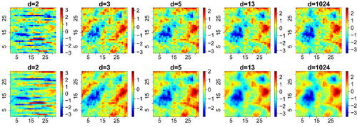
Fig. 2 Left: Root mean squared error of the composite likelihood estimator $\hspace{0.17em}\log \hspace{0.17em}({\widehat{\lambda }}_{C;d})$ (dashed lines) with $d=2,3,4,5$ (thin to thick) and cutoff distance δ = 2 (keeping about 10% of pairs), and the Vecchia likelihood estimator $\hspace{0.17em}\log \hspace{0.17em}({\widehat{\lambda }}_{V;d})$ (solid lines) with $d=2,3,4,5$ (thin to thick) and based on a coordinate ordering. Right: Relative efficiency of $\hspace{0.17em}\log \hspace{0.17em}({\widehat{\lambda }}_{C;d})$ with respect to $\hspace{0.17em}\log \hspace{0.17em}({\widehat{\lambda }}_{V;d})$ for $d=2,3,4,5$ (thin to thick). The Brown–Resnick model is considered here with parameters σ = 10 and $\lambda =1,\dots ,10$ (weak to strong dependence).

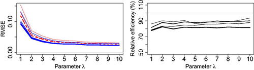
Table 1 Root mean squared error ($\times 100$) for the composite likelihood estimator $\hspace{0.17em}\log \hspace{0.17em}({\widehat{\lambda }}_{C;d})$ (left) with $d=2,3,4,5$ and cutoff distance $\delta =1,\sqrt{2},2$, and of the Vecchia likelihood estimator $\hspace{0.17em}\log \hspace{0.17em}({\widehat{\lambda }}_{V;d})$ (right) with $d=2,3,4,5$ and coordinate-based (p₁), random (p₂), middle out (p₃) and maximum–minimum (p₄) orderings.

	Composite estimator $\hspace{0.17em}\log \hspace{0.17em}({\widehat{\lambda }}_{C;d})$			Vecchia estimator $\hspace{0.17em}\log \hspace{0.17em}({\widehat{\lambda }}_{V;d})$
	cutoff distance δ			ordering
d	1	$\sqrt{2}$	2	p1	p2	p3	p4
2	3.08	3.43	3.86	3.34	3.93	3.56	4.54
3	—	3.08	3.34	2.82	3.05	2.83	3.18
4	—	2.93	3.17	2.79	2.81	2.77	2.87
5	—	—	3.31	2.69	2.71	2.68	2.70

NOTE: The Brown–Resnick model is here simulated with parameters σ = 10 and λ = 5 at D = 100 sites, with n = 100 replicates.

Table 2 Computational time (hr) for the composite likelihood estimator ${\widehat{\lambda }}_{C;d}$ (left) with $d=2,3,4,5$ and cutoff distance $\delta =1,\sqrt{2},2,\sqrt{5},\sqrt{8}$, and of the Vecchia likelihood estimator $\hspace{0.17em}\log \hspace{0.17em}({\widehat{\lambda }}_{V;d})$ (right) with $d=2,3,4,5$ and coordinate-based (p₁), random (p₂), middle out (p₃) and maximum–minimum (p₄) orderings.

	Composite estimator ${\widehat{\lambda }}_{C;d}$					Vecchia estimator ${\widehat{\lambda }}_{V;d}$
	cutoff distance δ					ordering
	1	$\sqrt{2}$	2	$\sqrt{5}$	$\sqrt{8}$	p1	p2	p3	p4
2	0.047	0.097	0.153	0.241${}^{\star }$	0.280${}^{\star }$	0.026	0.025	0.025	0.026
3	—	0.706	1.704	5.376${}^{\star }$	7.353${}^{\star }$	0.229	0.228	0.235	0.223
4	—	0.633	3.349	29.463${}^{\star }$	49.761${}^{\star }$	1.100	1.023	1.111	0.960
5	—	—	1.315	66.394${}^{\star }$	151.852${}^{\star }$	3.386	3.402	3.398	3.331

NOTE: The Brown–Resnick model is here simulated with parameters σ = 10 and λ = 5 at D = 100 sites, with n = 100 replicates. Numbers with an asterisk are extrapolated from the δ = 2 case by assuming that the computational time for ${\widehat{\lambda }}_{C;d}$ is proportional to the numbers reported in Table 1 of the supplementary materials.

Fig. 3 Left: Map of the study domain, with the spatial grid (dots) covering the Red Sea at which SST data are available. Ellipses show contours of the fitted extremal coefficient function $\widehat{\theta }(\mathit{h})=1.1,\dots ,1.9$, with respect to the grid cell at the center, obtained by fitting the anisotropic Brown–Resnick max-stable model using the best Vecchia likelihood estimator. Right: Validation locations (dots) used in our cross-validation study.

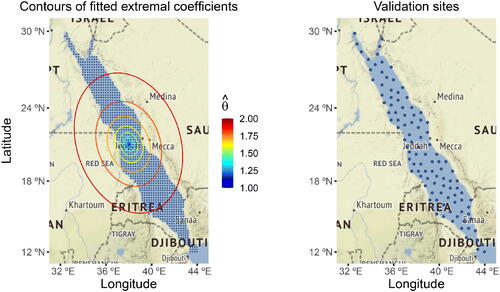
Table 3 Negative conditional log score S in (11) for each scenario based on a selection of 10% evenly spread validation locations.

	Vecchia					Composite
	Ordering	d = 2	d = 3	d = 4	d = 5	d = 2	d = 3	m
Anisotropic	p1	$97.6/92.5/107.7$	$96.6/91.6/107.1$	$97.7/91.4/113$	$98/91.4/112.7$	$130.1/\mathbf{115.9}/1053.6$	$125.8/117.6/946.3$	2
	p2	$101.4/93.2/118$	$97.7/91.6/105$	$100.6/91.4/105.5$	$97.3/91.5/105.1$	$129.8/117/1101.1$	$126/117/930.8$	4
	p3	$99.2/93.2/107$	$95.9/91.8/104.2$	$97.2/91.4/106.1$	$97.8/\mathbf{91.4}/105.2$	$129.7/117.4/1097.3$	$126.1/116.9/927.6$	6
	p4	$102.8/93.6/126.1$	$98/91.8/106.4$	$101.4/91.5/104.9$	$97.1/91.5/106.6$	$129.7/117.1/1061.7$	$126.3/116.9/929.5$	8
Isotropic	p1	$98/93.1/108.4$	$97.2/92.2/107$	$98.1/92/106.2$	$98.4/91.9/106.3$	$122.5/133.6/1088.4$	$\mathbf{117.7}/128.6/845.2$	2
	p2	$100.4/93/110.8$	$98.2/92.1/106.4$	$97.9/92/106.6$	$98.1/92/106.3$	$122.5/134.4/1101.6$	$117.7/128.4/841.4$	4
	p3	$98.1/93.2/108.1$	$96.5/92/106.9$	$97.5/\mathbf{91.9}/106.8$	$98.1/91.9/106.7$	$122.2/135.7/1124.6$	$117.8/128.4/840.4$	6
	p4	$101.7/92.8/114.4$	$98.5/92.2/106.8$	$97.6/92/106.6$	$97.9/92.1/107$	$122.3/135.8/1105.2$	$117.9/128.4/841.9$	8

NOTE: The three values in each cell correspond to $\alpha =0.5,1,1.5$, respectively. The best scenarios in each block (Vecchia/Composite × Anisotropic/Isotropic) are highlighted in bold. Orderings p₁, p₂, p₃, p₄ correspond to coordinate-based, random, middle-out, and maximum-minimum orderings, respectively. The maximum dimension of likelihood contributions is d (i.e., for Vecchia methods, with at most d–1 variables in the conditioning sets), and m relates to the cutoff distance for composite likelihoods.

Table 4 Computational time used in each scenario, measured in seconds.

	Vecchia					Composite
	Ordering	d = 2	d = 3	d = 4	d = 5	d = 2	d = 3	m
Anisotropic	p1	$201/24/120$	$1454/513/894$	$2790/2384/2051$	$6319/6699/9681$	$148/372/171$	$1266/1605/2304$	2
	p2	$329/155/152$	$796/469/527$	$1406/1703/2779$	$4796/6399/6928$	$573/377/335$	$2243/2442/3833$	4
	p3	$284/137/93$	$1026/459/868$	$3593/2245/2588$	$13670/5335/8566$	$480/548/565$	$3291/3381/3535$	6
	p4	$213/190/115$	$840/464/624$	$1836/2654/2330$	$9902/5032/7156$	$688/878/722$	$4972/4823/6493$	8
Isotropic	p1	$37/13/18$	$104/56/176$	$372/290/470$	$1136/829/1258$	$21/31/33$	$137/262/253$	2
	p2	$20/16/19$	$97/70/92$	$350/242/379$	$998/954/1056$	$39/56/58$	$417/452/462$	4
	p3	$19/13/30$	$97/73/84$	$340/273/414$	$1134/857/1442$	$55/81/90$	$501/613/623$	6
	p4	$19/12/18$	$101/62/84$	$370/218/332$	$1042/722/1179$	$69/100/108$	$560/937/843$	8

NOTE: For further details, see the caption of Figure 3.

Fig. 4 Binned bivariate empirical extremal coefficients (boxplots), plotted as a function of the Mahalanobis distance $d({\mathit{s}}_1,{\mathit{s}}_2)$, and their model-based counterparts (dashed curves) for the best anisotropic models obtained using the Vecchia likelihood approach (left) and traditional composite likelihood approach (right). The settings of these four “best models” can be read from Table 3.

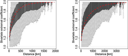
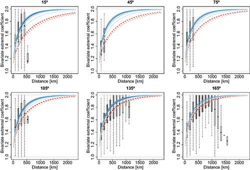
Fig. 5 Binned empirical extremal coefficients (boxplots) and their model-based counterparts (curves) for different directions, that is, ${15}^{°},{45}^{°},\dots ,{165}^{°}$ (subpanels from top left to bottom right), computed by fitting the best anisotropic models obtained with the Vecchia method (solid curves) and the composite likelihood method (dashed curves) based on sub-datasets of size $1,1/2,1/4,1/8,1/16\times 100\%$ of the complete dataset (light to dark). The different shades of gray of the binned boxplots correspond to the number of data points used in each boxplot, with darker gray corresponding to more points.