Fish early life stage toxicity prediction from acute daphnid toxicity and quantum chemistry

Figures & data

Figure 1. Distribution of pNOEC values as counts and normalized distribution functions a) for the chemicals in the training, DEV, and VAL set as defined in the Model development section, and b) according to their main pesticidal indication

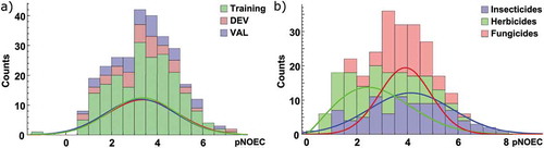
Table 1. Comparison of descriptor packages and their performance in training (r²) and cross-validation (q²) for a less complex model (3 latent variables (LVs) with 5 descriptors each) and a more complex model (5 LVs without regularization)

Software package	Number of descriptors	Number of descriptors without constant/correlated/missing	3 LVs à 5 descriptors		5 LVs, whole package
			r^2	q^2	r^2	q^2
CDK	223	132	0.512	0.401	0.610	0.400
RDKit	76	63	0.509	0.399	0.613	0.413
PaDEL	1875	891	0.581	0.421	0.778	0.415
Dragon	5270	1714	0.573	0.372	0.749	0.447
QM	40	19	0.511	0.450	0.535	0.452
MACCS	167	126	0.340	0.148	0.447	0.101
Morgan	1024	390	0.192	0.039	0.230	0.054
Unity	992	843	0.296	0.082	0.584	0.058
ALL	9667	4178	0.642	0.391	0.801	0.455

Figure 2. Goodness of fit (r²) and cross-validated q² of sPLS models with increasing numbers of latent variables (LV) and descriptors per LV from the packages CDK, RDKit, PaDEL, Dragon, QM, and pEC50 daphnid

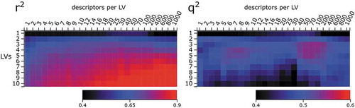
Figure 3. Average similarity to the 5 most similar compounds from the training set, based on Tanimoto distance of Unity fingerprints. For the training (left) and DEV (right) sets, all compounds from the training set were considered, while for the cross-validation (middle) only compounds from the other CV-batches were considered

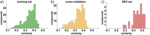
Table 2. Model performance summary along the major development steps, starting from all descriptors (CDK, RDKit, PaDEL, Dragon, QM and pEC50 daphnid) and gradually refining the model while reducing its complexity

Model	#LV/#descr.	r^2	q^2	r^2dev	RMSE (training)	RMSE (cross-val.)	RMSE (DEV)
M1, PLS with all descriptors	2/2225	0.554	0.463	0.452	0.961	1.060	1.025
M2, sPLS with max. q^2 (3x100)	3/294	0.693	0.546	0.493	0.798	0.986	0.986
M3, sPLS local max. q^2 (4x7)	4/27	0.698	0.534	0.647	0.791	1.048	0.822
M4, sPLS pre-selection (10x5)	10/50	0.815	0.415	0.632	0.618	1.100	0.840
M5, manual refinement	3/18	0.757	0.694	0.700	0.709	0.775	0.758
M6, manual refinement	2/9	0.723	0.686	0.729	0.757	0.808	0.720

#LV/#descr: number of latent variables (LVs) and descriptors, e.g. the sPLS model with 3 LVs and 100 descriptors each (‘3x100ʹ) has nearly 300 descriptor variables in total. Descriptor variables may be selected for multiple latent variables.

r², q², RMSE as explained in Materials and methods section.

Table 3. Model coefficients (c_i) and descriptors for use with equation 3(3) $\mathrm{p}\mathrm{N}\mathrm{O}\mathrm{E}\mathrm{C}=-log\left(NOEC\left[mM\right]\right)=a+\sum c_i{d}_i$(3) and model M6 (for more detailed descriptions see Table S2 in the Supporting Information)

ci (norm.)	Descriptors i	Description	Class
– 0.236367	hBondacceptors_CDK2	Number of hydrogen bond acceptor sites	1D
0.193715	HATS1p_Dragon	Leverage-weighted autocorrelation of lag 1/weighted by polarizability (GETAWAY 3D-autocorrelation)	3D
0.490086	ALOGP_Dragon	Ghose-Crippen octanol-water partition coeff. (logP)	2D
0.236732	DLS_03_Dragon	Modified drug-like score from Walters et al. (6 rules)	1D
0.213228	PolarisabilityAnisotropy_QM	Anisotropy of the static polarizability tensor	3D
– 0.333269	COSMORS_Hacc_QM	COSMO-RS hydrogen bond acceptor moment	3D
0.266294	slogp_VSA3_RDKit	Van der Waals surface area with logP from −0.20 to 0.00	2D
0.328670	smr_VSA4_RDKit	Van der Waals surface area with molecular refractivity from 2.24 to 2.45	2D
0.518995	pEC50 daphnid	Daphnid acute (48 h) EC50 endpoint, neg. log.	exptl.
3.445870	constant a

Figure 4. Loadings plot of the 9 descriptors and pNOEC for the two latent variables in model M6. See descriptor explanations in Table 3

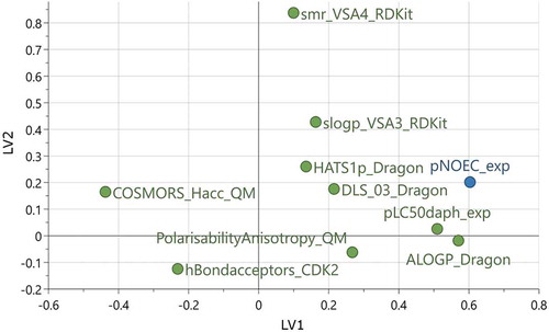
Figure 5. Model M6: Predictions with confidence intervals vs. experiment, for the training set compounds (a) and test sets (b), coloured in red (DEV), blue (VAL), and grey (EXT)

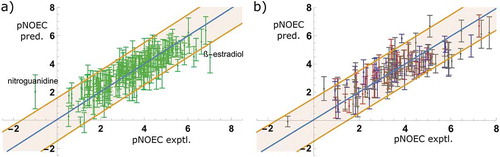
Figure 6. Error distribution of pNOEC predictions by model M6 as counts and normalized distribution functions a) according to set membership and b) for pesticide classes

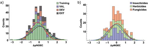
Figure 7. Error distribution of pNOEC predictions for pesticides by model M6, coloured according to mode of action (for an explanation of MoA acronyms see SI Table S8, and Figures S6-S8 for histograms on individual MoAs)

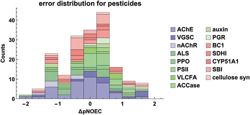
Figure 8. Cook’s distances for the training and test sets (n = 338) for PLS model M6

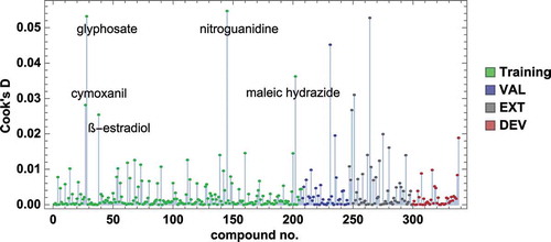
Figure 9. Williams plot with 5 influential training set compounds from Cook’s plot marked

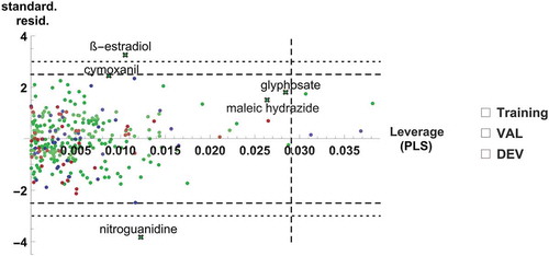
Figure 10. Representation of the chemical space covered by the full data set with 338 molecules. We used a t-stochastic neighbour embedding (tSNE) based on Tanimoto distances to embed chemical similarities in two dimensions. Training set (orange) and test set (blue) compounds of the models by Furuhama et al. highlighted in colour

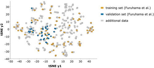
Table 4. Comparison of QSAAR model performance with models by Furuhama et al. [15]

	ID 1 ^a)	ID 2 ^a)	ID 3 ^a)	ID 4 ^a)	Ct432 ^a)	QAAR ^a)	M6 (this work)
RMSEext ^b)	0.89	0.91	0.93	0.87	0.63	0.64	0.62
r^2ext ^c)	0.38	0.39	0.36	0.52	0.56	0.56	0.63
Q^2ext ^d)	0.16	0.12	0.09	0.20	0.58	0.57	0.57
z > 1.0 ^e)	8	8	7	6	2	2	1
RMSEVAL‘ ^f)	1.04	0.99	1.14	1.27	1.14	1.20	0.79
r^2VAL‘ ^f)	0.50	0.54	0.40	0.26	0.39	0.28	0.69
no. of variables	8	9	9	7	2	1	9
proprietary software required	yes	yes	yes	yes	no	no	yes

^aID 1–4, Ct432, QAAR are models with the lowest errors from ref [15]. Results in rows 1–4 were taken from the original article for comparison.

^bRMSE_ext, root mean square error on validation set from ref [15].

^cr²_ext, squared correlation coefficient between measured and estimated pNOEC on validation set from ref [15].

^dQ²_ext, external explained variance on validation set as given in ref [15].

^ez > 1.0, number of underestimates by more than 1 log unit on validation set from ref [15].

^fRMSE_VAL’, r²_VAL’ on validation set from this work, excluding compounds with missing values for daphnids. 4 chemicals were present in the training set of models ID1-4, Ct432, QAAR.

A. Furuhama, T.I. Hayashi, and H. Yamamoto, Development of models to predict fish early-life stage toxicity from acute Daphnia magna toxicity, SAR QSAR Environ. Res. 29 (2018), pp. 725–742. doi:10.1080/1062936X.2018.1513423.

 PubMed Web of Science ®Google Scholar

Data availability Statement

The data that support the findings of this study are openly available via figshare at http://doi.org/10.6084/m9.figshare.c.5194022. The model workflow is available in KNIME Hub at https://kni.me/w/CEyXPUo_n1i4pUiR.