Figures & data
Figure 1. Number of publications addressing MPC of urban drainage systems per 5 years.
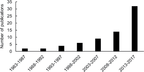
Table 1. RTC terms. Physical devices in italic and bold and their modeling counterparts in italic.
Table 2. Categorization of control methods.
Figure 2. The concept of MPC, including the receding horizon principle and optimization. The terms “prediction horizon” and “sampling interval” are explained in Section 3. TOF = time of forecast.
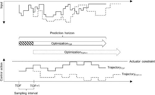
Table 3. Overview of terminology used in this review and in the literature and definitions of the term.
Figure 3. Hierarchical categorization of MPC components. A solid line indicates that a component consists of subcomponents, while a dashed line indicates the presence of an external subcomponent. The color scheme can be used as a reading guide for the remaining part of the paper.
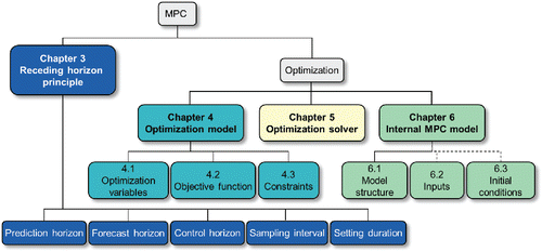
Figure 4. Time windows used in the receding horizon principle. The lengths of the time windows are only an example. Here, the sampling time is twice as long as the setting duration, as in . Inspired by Rauch and Harremoës (Citation1999).
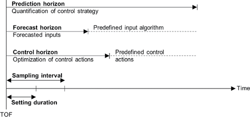
Figure 5. The difference between the collective horizon, sampling interval, and setting duration. In (a) the sampling interval is longer than the setting duration; in (b) they are equally long; and in (c) the sampling interval is shorter.
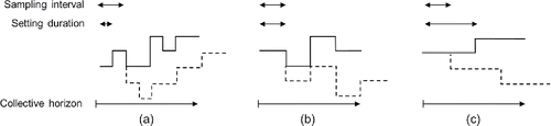
Table 4. Commonly applied objectives, operational goals, and associated metrics.
Table 5. Description of model elements used in internal MPC models.
Table 6. Overview of the model elements included in the internal MPC models for some of the reviewed literature. The use of an element is indicated with ✓ and the ability to model backwater effects (backwat.) and internal (int.) and external (ext.) overflows is noted. The linearity of the internal MPC model is also shown.
Table 7. Model techniques applied for different linear model elements.
Figure 6. Relation between a HiFi model and an internal MPC model and its input, exemplified for a catchment in Copenhagen, Denmark. (a) The HiFi model used as starting point. (b) The relevant part of the HiFi model containing the sewer system affected by the control optimization, which may contain backwater effects and internal and external overflows. (c) The conceptual, internal MPC model of the relevant part of the sewer system with flow input from measurements or generated by a (simplified or HiFi) input model.
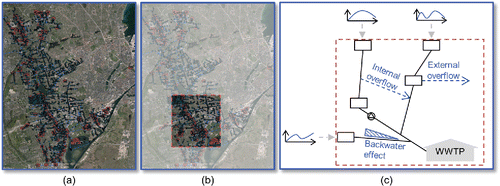
Figure 7. Different routes to take from control problem to optimal control actions.
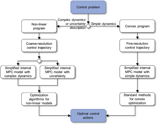
Figure 8. Time-scale dependent control hierarchy for sewer systems. The indication of control strategies used at each layer in the hierarchy is slightly modified from Mollerup et al. (Citation2017) based on the terminology and structure developed in this review.
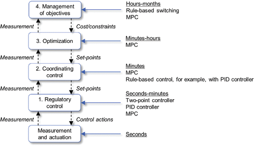
Table 8. MPC performance reported by the reviewed literature. A performance span for all applied rain events is stated together with the overall improvement for these events (written in []), if possible. Only one of the two is shown if information is scarce or only one rain event is considered.
Table 9. Checklist for writing MPC papers within urban drainage. Example literature is given where [1] Vezzaro and Grum (Citation2012) is a conference article containing less information than the journal article [2] Vezzaro and Grum (Citation2014). ✓ means that the information is included, (✓) that it is partly included, ✗ that it is missing, and n.r. that it is not relevant information in this specific paper.