A four-dimensional inversion of the acoustic tomography, satellite altimetry and in situ data using Quasigeostrophic constraints

Figures & data

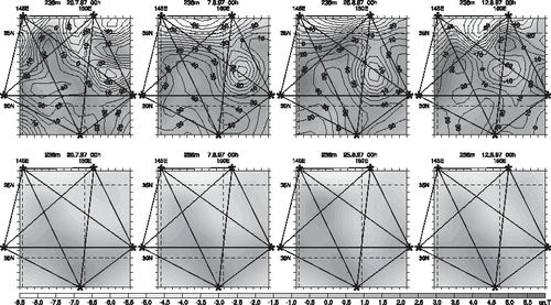
FIGURE 1 Climatological distribution of the seawater density at 236 m in the Kuroshio Extension region. Positions of the acoustic transceivers are given by asterisks and correspond to the configuration of the real AT array maintained in the region for 2 months in 1997. Sloping dashed lines denote satellite tracks along which sea surface height is measured. Solid lines symbolically show the tracks of acoustic rays. Bold lines give the area “best covered” by the acoustic tomography. Density contours are in 10⁻² kg/m³.

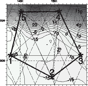
FIGURE 2 Evolution of the cost function (dashed line) and the norm of the gradient (solid line) with iteration number. Both quantities are normalized by their initial values.

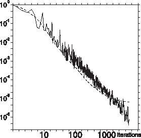
FIGURE 3 Difference between the density fields of the reference and the model solutions at 414 m before (upper panels), and after the inversion. Contour interval is 0.05 kg/m³.

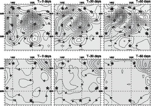
FIGURE 4 Quality of inversion q* as a function of the noise level ε for the cases of AT travel time (solid lines) and differential travel time observations. Curves with larger (smaller) q* were computed for the cases of K = 250 (125) rays. SSH noise level ε_ζ = 0.05 was kept constant.

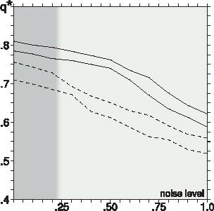
FIGURE 5 Quality of inversion q* as a function of depth for various types of data sets (a) and their combinations; (b) Curves in the left panel correspond to the inversions of travel times δτ_ρ (1); differential travel times δτ_ψ (2); altimetry (3); density (4); and current velocity (5); observations. Curves on the right correspond to the inversions of the following combinations of data: δτ_ρ (4); δτ_ρ and δτ_ψ (2); δτ_ρ and (3); and all types of observations (curve 1). Note that the formal shares of altimetry (3.6%), density (1.0%) and velocity (0.6%) data points in the total amount are much smaller than their relative contributions to the improvement of q*.

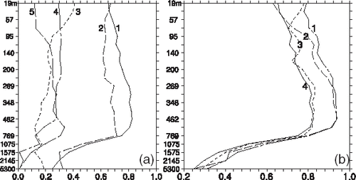
TABLE I Assimilation quality computed for the ray systems with different number of rays K and vertical position h of the transceivers. Superscripts denote data types (travel times TT or differential travel times DT) used in the experiments

K	h(m)	η	M
250	1050	0.037	10.2	0.78	0.84	0.80	0.69
126	1050	0.056	8.01	0.62	0.69	0.67	0.48
125	1050	0.072	9.97	0.76	0.82	0.74	0.66
41	1050	0.156	6.24	0.58	0.52	0.58	0.43
125	300	0.055	7.79	0.57	0.65	0.57	0.39
125	500	0.053	7.57	0.63	0.71	0.68	0.47
125	2100	0.062	8.63	0.62	0.74	0.64	0.48

TABLE II Results of the inversion experiments with fixed regularization and varying first guess

α	d
1.0	0.000	0.78	0.71
0.8	0.008	0.77	0.70
0.5	0.018	0.76	0.65
0.3	0.051	0.73	0.59

TABLE III Identification of the ray paths. The number of identified rays N is shown for each station pair. The ray bundles are characterized by their temporal mean travel times ⟨τ⟩, the corresponding rms variances , and the rms misfits between the mean measured travel times and those computed using the time-invariant background sound slowness distribution. Error bars show variations of the corresponding quantities within the bundle. Note relatively large travel time variances for the pairs containing stations 4 and 5 located across the KE front (Fig. 1)

Station pair	N	⟨τ⟩, s	σ(τ), ms	ms
1–2	16	448.3 ± 0.6	76 ±  6	6
1–3	20	666.2 ±  0.9	26 ±  2	14
1–4	17	608.0 ±  0.8	124 ±  4	133
1–5	14	416.3 ±  0.6	169 ±  19	67
2–3	15	343.0 ±  0.5	66 ±  3	8
2–4	18	615.8 ±  0.8	120 ±  9	103
2–5	17	673.0 ±  0.8	83 ±  5	91
3–4	16	453.7 ±  0.6	118 ±  4	96
3–5	18	682.7 ±  0.8	157 ±  7	94
4–5	11	342.6 ±  0.5	189 ±  29	37
Total	162	–	107 ±  7	70

FIGURE 6 Evolution with time of the tomography (solid lines, left axis) and differential tomography (dashed lines, right axis) model/data misfits. Curves 1 and 2 correspond to errors of the first-guess solution. Mean prior error variance levels are shown by thick horizontal lines. Curves 3 and 4 are those obtained after the DCI. Long dashed line 5 (left axis) shows evolution of the travel time error obtained by the LSI method.

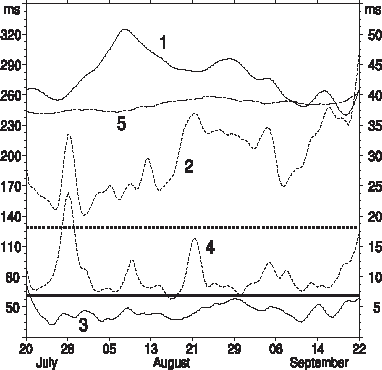
FIGURE 7 Temperature section along (T2–T5) line as measured on July 20–22 by CTD hydrocasts (a) and obtained as a result of the DCI (b), and LSI (c) methods.

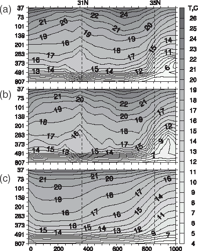
FIGURE 8 Comparison of the evolution of temperature anomalies (gray color) inferred from the dynamically constrained inversion (upper panels) with the anomalies obtained by the 3D LSI method of the same travel time data. Stream function is available only for the DCI solution and is shown by contours (in 1000 m²/s).