Figures & data
Figure 1. Time evolution of the 2D plume profile. (a) Exact distribution and (b) recovered distribution.
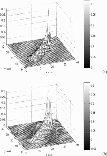
Figure 2. Exact and recovered concentration profiles at (a) 20%, (b) 40%, (c) 60%, and (d) 80% backwards in time.
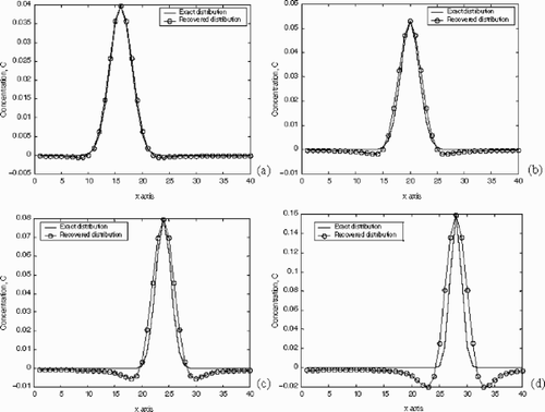
Figure 3. Evolution of the mass error.
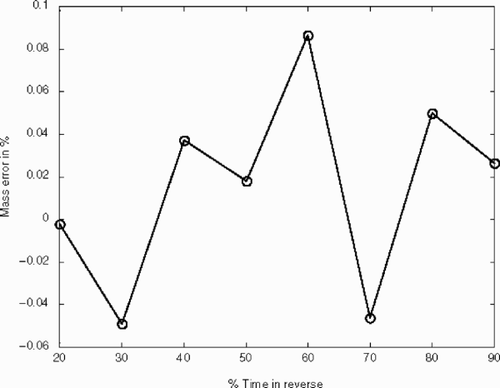
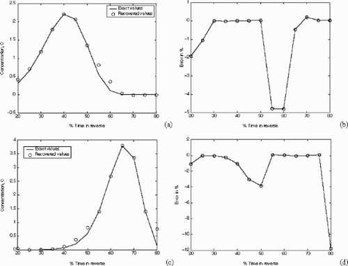
Figure 4. Evolution of the concentration at the single mobile observation or conditioning point.
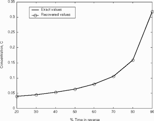
Figure 5. Evolution of the total error, which is a weighted sum of the mass error and the point concentration error.
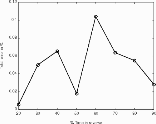
Figure 6. Evolution of the 2D plume profile (initial, 20, 40, 60 and 85% back in time). (a) Exact distribution and (b) recovered distribution.
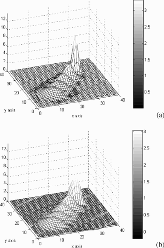
Figure 7. Snapshots of 2D plume in the form of contours (initial, 20, 40, 60 and 85% back in time). (a) Exact distribution and (b) recovered distribution. Observation points are identified as stars (*) and concentration contours are shown only at the 1, 2, 3, 4, 4.5, 5, 5.5, and 6 levels.
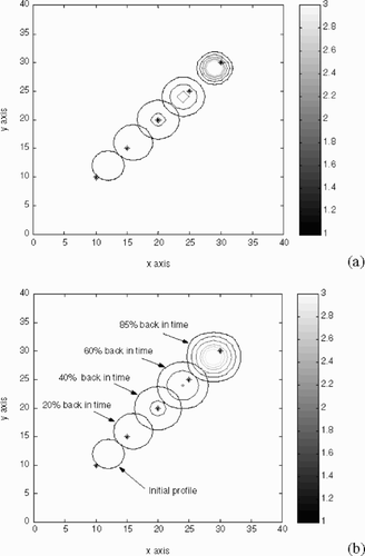
Figure 8. Exact and recovered concentration profiles at (a) 20%, (b) 40%, (c) 60%, (d) 80%, and (e) 85% backwards in time.
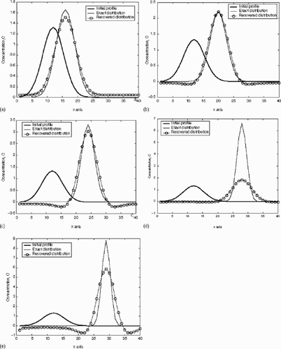
Figure 9. Time evolution of the (a) mass balance and (b) total error involved in the reconstruction.
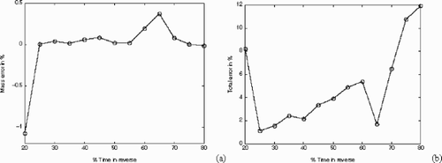
Figure 10. Evolution of objective function for the reconstruction at 20% backward in time.
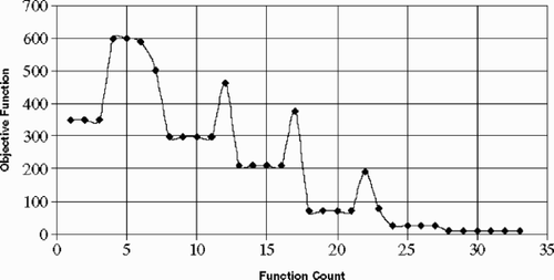
Figure 11. Breakthrough curve and corresponding evolution of the error at the conditioning point located at (a) and (b) (20, 20), and (c) and (d) (25, 25).