Transient and steady state free convection from a horizontal cylinder

Figures & data

Table I Experimental conditions

Measurement	Range	σ
Heat flux Q/A	2100 W/m^2	3 W/m^2
Ts	295–417 K	0.1 K
Ts − Ta	2–120 K	0.2 K

Figure 1 (a) Temperature history; (b) Heat flux history.

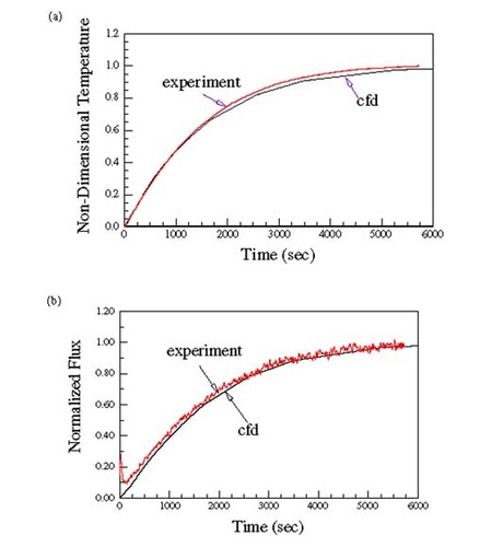
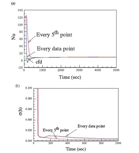
Figure 2 Nusselt Numbers estimated by the function specification method with r = 5 and from the cfd simulation.

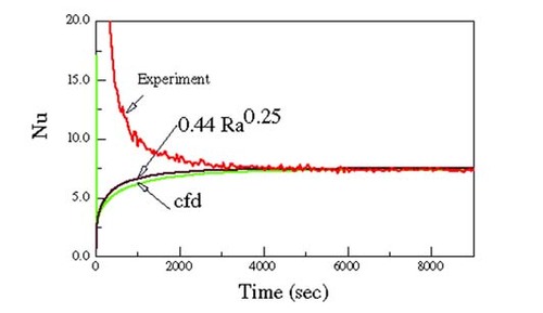
Figure 3 (a) Typical time history of the ambient temperature; (b) autocorrelation coefficient for the ambient temperature shown in Fig. 3(a).

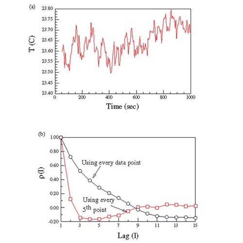
Table II Standard deviation of the average T_a

Sampling rate	Full W	Diagonal W	Ratio
Every date point	0.1266	0.0567	2.23
Every 5th point	0.0520	0.0513	1.01

Figure 4 σ(h_ss) as a function of the function specification parameter r.

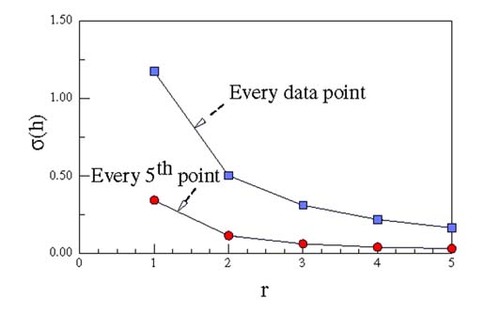
Figure 5 Time history of: (a) σ(T); (b) σ(h).

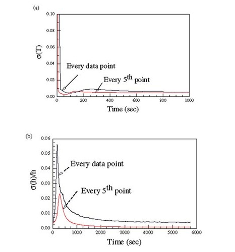
Figure 6 Estimated surface heat flux showing the effect of considering heat losses, L and errors in the energy stored, S.

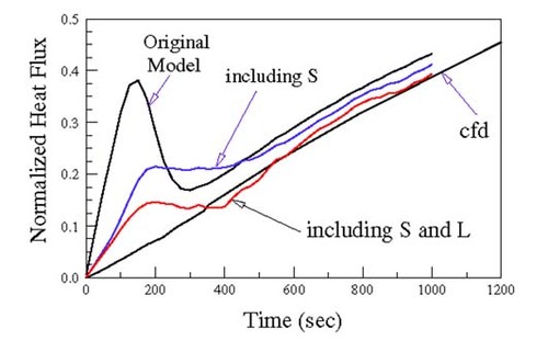
Figure 7 (a) History of h for the new system computed using the Kalman filter; (b) history σ(h) for the new system computed using the Kalman filter.

Table

A	surface area
B	matrix
D	cylinder outside diameter
E ( )	expected value
h	convective heat transfer coefficient
(---535----14)	mean value of h
hss	steady state h
k	thermal conductivity of the air
J	least squares function
l	lag
L	heat loss
Nu	Nusselt number (hD/k)
Q	heat supplied by heater
r	function specification method parameters
Ra	Rayleigh number
S	error in heat stored
t	time
Δt	sampling time
Ta	ambient temperature
Ts	surface temperature
x	column vector
x^T	transpose of x
y	state variable vector
(---535----15)	estimated value of y
(---535----16)	conditional expectation
σ()	standard deviation
W	covariance matrix of noise
∑	covariance matrix of the errors in the state variables