Teaching Prediction Intervals

Figures & data

Figure 1. Gaps Between Consecutive Ordered Observations. This diagram draws attention to the gaps between consecutive ordered observations in a sample of size 19. The next observation is equally likely to occupy each of these 20 gaps.

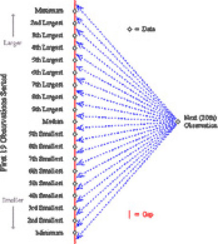
Table 1. Failure Times of 19 Randomly Sampled Components

Failure time (sorted)
32.56	42.02	47.26	50.25	59.03	60.17	61.56	62.16	62.84	63.29
63.52	65.52	66.54	68.71	70.60	71.27	76.33	80.37	87.87

Figure 2. Dotplot of Failure Times. A dotplot of the failure time data of Table 1 is displayed. One-sample nonparametric prediction intervals are shown for a variety of levels.

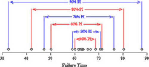
Figure 3. Applying the Nonparametric PI in Simple Linear Regression. A scatterplot of energy consumption versus size of residence for 40 residences is displayed. The least squares fit and boxplots for both energy consumption (univariate) and the residuals are shown. A one-sample nonparametric 50% PI for the residuals is bounded by the first and third quartiles. This interval is then applied to the fitted line to obtain a prediction band. 50% of the observations lie within this band.

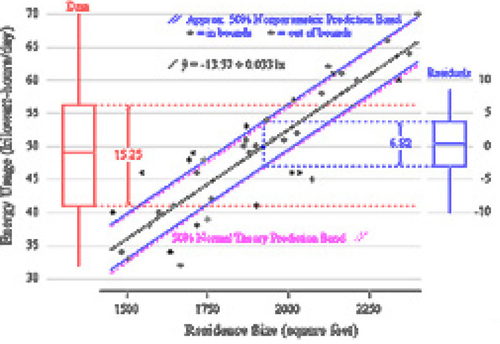
Figure 4. The PI Fails when Variance is Not Constant. A scatterplot of systolic blood pressure versus age, for healthy women, is displayed. The nonparametric PI is applied with the residuals to obtain a 50% prediction band. Because of nonconstant error variance, the band fails to predict at the 50% level for all ages.

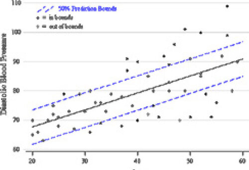
Table 2. Nonparametric and Normal Theory Prediction Bounds for Component Failure Times

	Prediction Bounds
	Lower	Upper
Level	Nonparametric	Normal	Nonparametric	Normal
90%	32.56	39.46	87.87	86.00
80%	42.02	44.88	80.37	80.58
70%	47.26	48.41	76.33	77.05
60%	50.25	51.16	71.27	74.30
50%	59.03	53.49	70.60	71.97
40%	60.17	55.57	68.71	69.89
30%	61.56	57.48	66.54	67.98
20%	62.16	59.28	65.52	66.18
10%	62.84	61.02	63.52	64.44
0%	63.29	62.73	63.29	62.73

NOTE: The nonparametric bounds are simply the data presented in Table 1. The normal theory bounds are obtained using (6) and (7) with $\overline{y}$ = 62.730 and s = 13.077.

Figure 5. Plotting Corresponding Prediction Interval Bounds. A plot of nonparametric prediction bounds versus normal theory counterparts is shown for the component failure time data. The bounds are listed in Table 2. A normal probability plot is superimposed:

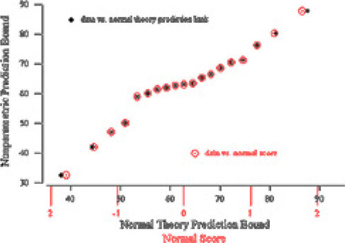
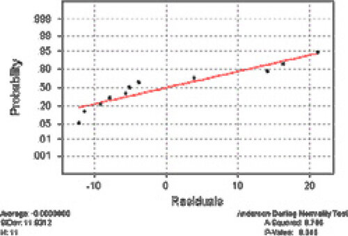
Figure 6. Normal Probability Plot of Residuals. Price of the Orion model automobile is regressed on age; a normal probability plot of the residuals is displayed.