663
Views
0
CrossRef citations to date
0
Altmetric
Original Articles

Teaching Statistical Concepts with Student-Specific Datasets

Figures & data

Figure 1 Histogram of 144 students' test statistics , where is the mean of n = 25 observations, pseudo-randomly generated from the normal distribution with mean μ = 135 and standard deviation σ = 20. Histogram is plotted against the t distribution with n − 1 = 24 degrees of freedom. Figure demonstrates the behavior of the test statistic when , is true.
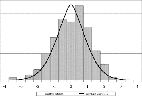
Figure 1 Histogram of 144 students' test statistics , where is the mean of n = 25 observations, pseudo-randomly generated from the normal distribution with mean μ = 135 and standard deviation σ = 20. Histogram is plotted against the t distribution with n − 1 = 24 degrees of freedom. Figure demonstrates the behavior of the test statistic when , is true.

Figure 2 Histogram of 144 students' test statistics , where is the mean of n = 25 observations, pseudo-randomly generated from the normal distribution with mean μ = 135 and standard deviation σ = 20. Histogram is plotted against the t distribution with n − 1 = 24 degrees of freedom. Figure demonstrates the behavior of the test statistic when is false.
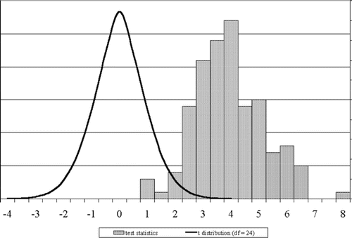
Figure 2 Histogram of 144 students' test statistics , where is the mean of n = 25 observations, pseudo-randomly generated from the normal distribution with mean μ = 135 and standard deviation σ = 20. Histogram is plotted against the t distribution with n − 1 = 24 degrees of freedom. Figure demonstrates the behavior of the test statistic when is false.
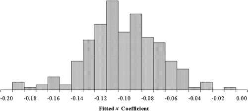
Figure 3 Histogram of students' fitted parameters, when each student fit the model to n = 15 (x, y) observations drawn from y = 10000 − 0.10 x + ε. ε is normally distributed with mean 0 and standard deviation σ= 800.

Figure 3 Histogram of students' fitted parameters, when each student fit the model to n = 15 (x, y) observations drawn from y = 10000 − 0.10 x + ε. ε is normally distributed with mean 0 and standard deviation σ= 800.

Figure 4 at x = 40,000. (E[y | x = 40,000] = 10,000 − 0.10 (40,000) = 6,000).

Figure 4 at x = 40,000. (E[y | x = 40,000] = 10,000 − 0.10 (40,000) = 6,000).

Reprints and Corporate Permissions

Please note: Selecting permissions does not provide access to the full text of the article, please see our help page How do I view content?

To request a reprint or corporate permissions for this article, please click on the relevant link below:

Academic Permissions

Please note: Selecting permissions does not provide access to the full text of the article, please see our help page How do I view content?

Obtain permissions instantly via Rightslink by clicking on the button below:

If you are unable to obtain permissions via Rightslink, please complete and submit this Permissions form. For more information, please visit our Permissions help page.