Figures & data
Figure 1: Scatterplot of retail price and mileage.
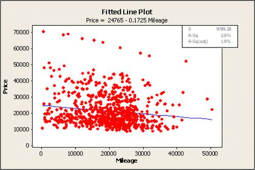
Figure 2: Output from the best subsets technique in Minitab. Only the best two models for each number of variables (Vars.) are displayed.
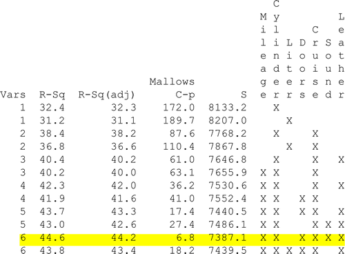
Figure 3: Residual plots for Equation 2.
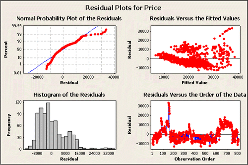
Figure 4: A residual versus order plot using Equation 1: Price = 24723 — 0.17 Mileage.
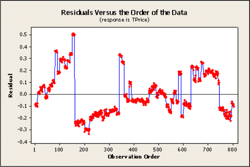
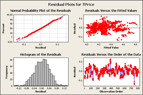
Figure 5: Minitab plots of the residuals for the Equation 3: TPrice = 3.98 – 0.000003 Mileage + 0.0997 Liter + 0.0400 Buick + 0.249 Cadillac – 0.00937 Chev + 0.0136 Pontiac + 0.345 SAAB. The histogram and normal probability plot show that the error terms are not normally distributed. The plot of Residuals vs. Fitted values looks better but some clustering is still visible. The Residuals vs. Order plot also shows some systematic patterns, but they are much less pronounced than before.
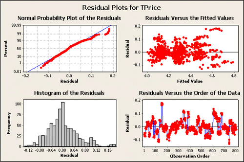
Figure 6: Residual plots for Equation 4: a multivariate regression model to predict TPrice with Make, Trim, Mileage, Liter, Doors, Cruise, Sound, and Leather as explanatory variables. The residuals appear to be homoskedastic and more closely follow a normal distribution. The Kolmogorov-Smirnov (K-S) test for normality resulted in a p-value = 0.13. The residual vs. order plot has much less clustering. Students may want to consider including Model as a predictor, but the corresponding set of dummy variables is very large, and adding them to the model doesn't improve R-Sq.