Figures & data
Figure 1: SOCR LLN APplet interface.
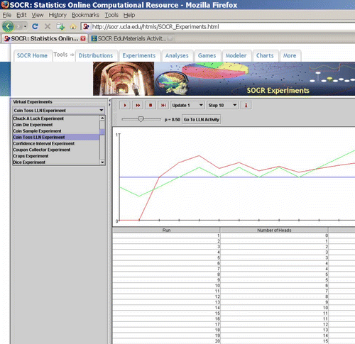
Figure 2: SOCR LLN Activity: Snapshot of the first experiment.
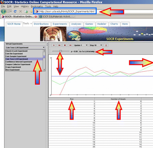
Figure 3: Interactive applet demonstration of the two common LLN misconceptions. First, the outcome of each experiment is independent of the previous outcomes. Second, the variable representing the raw difference between the number of Heads and Tails is divergent, unstable and unpredictable. The top panel shows a simulation with only 100 trials. The bottom panel shows an outcome with 10,000 simulations. Notice the rapid convergence of the red curve (proportions), the expansion of the vertical scale on the right side and the vertical graph compression of the variable that follows with such a large increase in the number of trials.
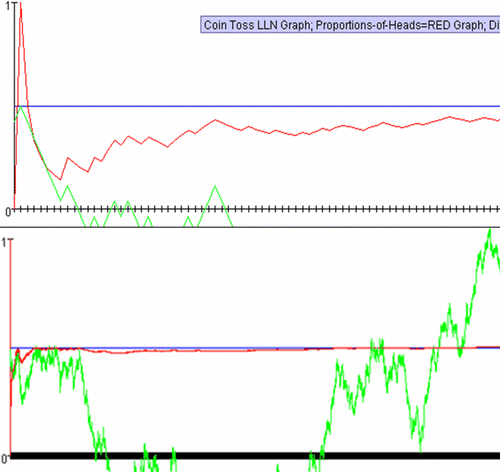
Figure 4: SOCR LLN Activity: Snapshot of the second (Binomial coin) experiment.
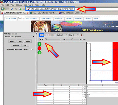
Figure 5: Demonstration of the LLN using the Binomial coin experiment. As we increase the number of experiments (N) from 10 (top) to 100 (middle) and then to 1,000 (bottom), we observe a better match between the theoretical distribution (blue graph) and the empirical distribution (red graph). In this case, we used number of coin-tosses n=27 and p=P(H)=0.7. According to the LLN, the same behavior can be demonstrated for any choice of these Binomial parameters.
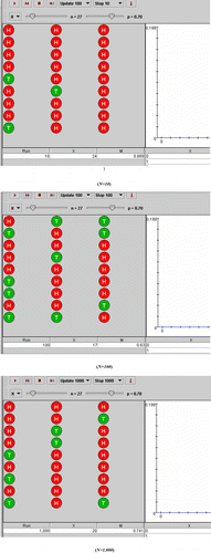
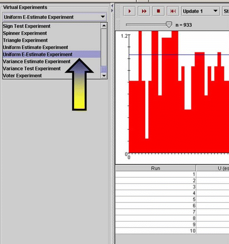
Figure 6: SOCR Uniform E-Estimate applet illustrating the stochastic approximation of e by random sampling from Uniform(0,1) distribution.