Figures & data
Fig. 1 Output of P.sim(3), simulated outcomes of two four-sided dice rolls. (Note that Python uses zero-based indexing.)
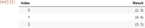
Fig. 2 Approximate distribution of Y, the maximum of two four-sided dice rolls (table and plot).
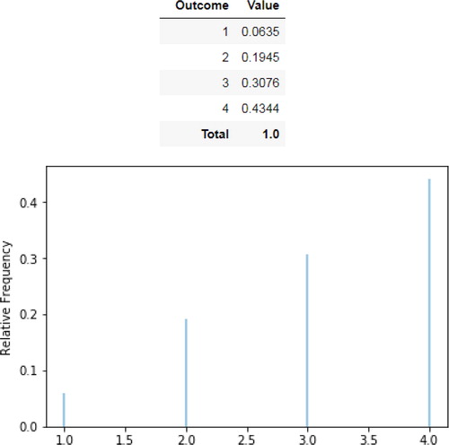
Fig. 3 Approximate joint and marginal distributions of X and Y, the sum and maximum of two four-sided dice rolls.
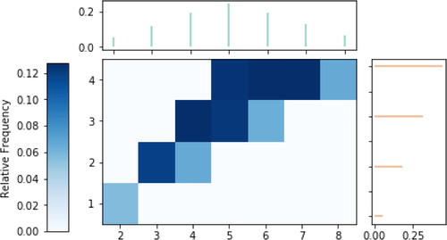
Fig. 4 Sample paths of a Poisson process with rate parameter 1.
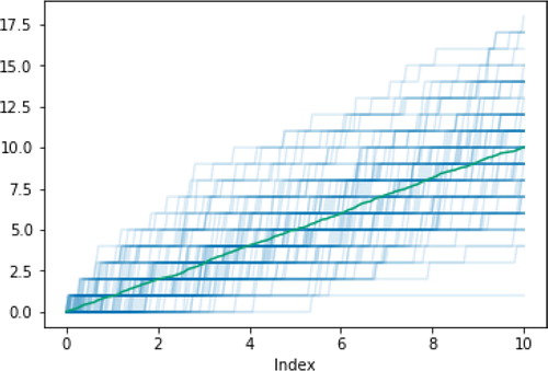
Fig. 5 Approximate joint and marginal distributions of , the process value at time 1.5, and T2, the time of the third arrival, for a rate 1 Poisson process N.
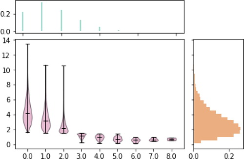
Fig. 6 Ten sample paths of a simple symmetric random walk on the integers.

Fig. 7 Kernel density plot of simulated values of .
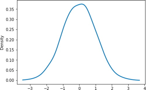
Fig. 8 Simulated outcomes of independent dice rolls.
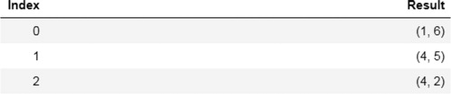
Fig. 9 Simulated realizations of the event , where
, X and Y are independent,
, and
.
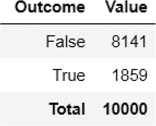
Fig. 10 Approximate conditional distribution of X given .
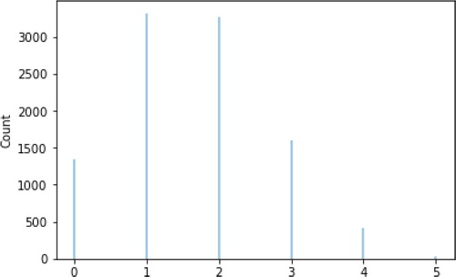
Fig. 11 Log transform of a random variable with a Uniform(0,1) distribution.
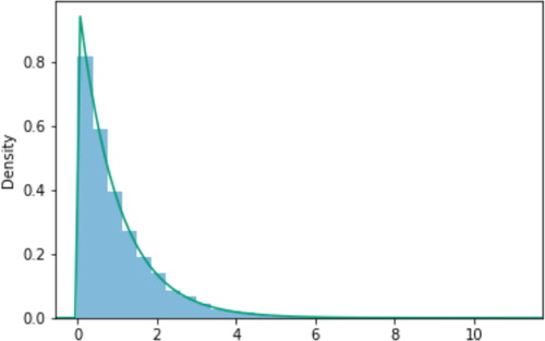
Table 1 Comparison of Symbulate and R commands for the example illustrated in .
Fig. 12 Superimposed histograms.
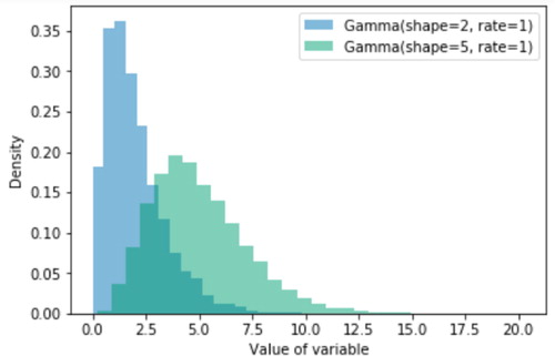
Fig. 13 Bivariate normal distribution: joint and marginal densities.
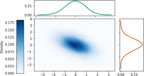
Fig. 14 Joint and joint conditional distributions for Example 2.
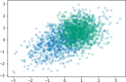
Fig. 15 Sample paths of an Ornstein–Uhlenbeck process.
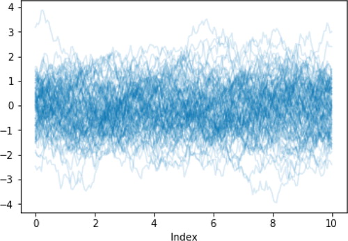
Table 2 Symbulate commands.
Table 3 Comparison across packages of syntax for a Normal(0, 1) distribution.
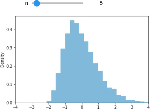
Fig. 16 Sampling distribution of the standardized sample mean, with a slider for n (n = 5 is displayed).