A Comparison of Different Approaches for Estimating Cross-Lagged Effects from a Causal Inference Perspective

Figures & data

Figure 1. Causal diagram that shows the relationship between the covariates, the exposure $X_s,$ and the outcome $Y_t.$ ${\mathrm{\tau }}_{{\mathcal{T}}_{X,Y,L},\mathrm{ACE}}$ denotes the average causal effect (ACE) of $X_s$ on $Y_t.$

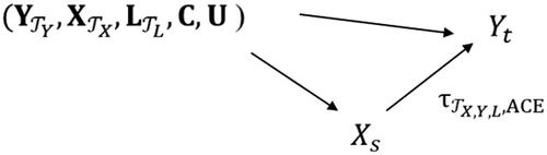
Figure 2. Path diagrams of the cross-lagged panel models with lag-1 (CL1) and lag-2 (CL2) effects for three measurement waves.

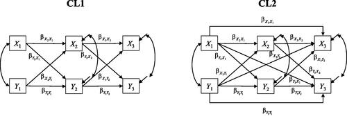
Figure 3. Path diagram of an observation-level model with a single latent variable (OL1; Finkel, 1995) for three measurement waves.

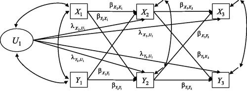
Figure 4. Path diagram of an observation-level model with two latent variables (OL2; Dishop & DeShon, 2021; see also Bollen & Brand, 2010) for three measurement waves.

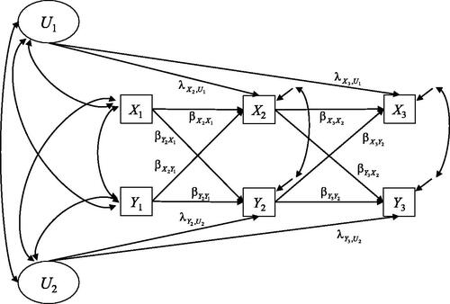
Table 1. Overview of different latent variable-type models that adjust for effects of unmeasured variables $\mathbf{U}.$

		Effects of $\mathbf{U}$
Model	Dimension $\mathbf{U}$	Time 1	Time 2 and 3	Coefficients
Observation-Level
OL1	1	$\mathrm{Cov}\left({\mathbf{Z}}_1,\mathbf{U}\right)={\mathbf{\Psi }}_{{\mathbf{Z}}_1\mathbf{U}}$	${\mathbf{\Lambda }}_2\ne {\mathbf{\Lambda }}_3$	${\mathbf{B}}_{21}={\mathbf{B}}_{32}$
OL2	2	$\mathrm{Cov}\left({\mathbf{Z}}_1,\mathbf{U}\right)={\mathbf{\Psi }}_{{\mathbf{Z}}_1\mathbf{U}}$	${\mathbf{\Lambda }}_2$ and ${\mathbf{\Lambda }}_3$ diagonal; ${\mathbf{\Lambda }}_2={\mathbf{\Lambda }}_3$	${\mathbf{B}}_{21}={\mathbf{B}}_{32}$
OL3	2	${\mathbf{\Lambda }}_1$ diagonal	${\mathbf{\Lambda }}_2$ and ${\mathbf{\Lambda }}_3$ diagonal;${\mathbf{\Lambda }}_2={\mathbf{\Lambda }}_3$	${\mathbf{B}}_{21}={\mathbf{B}}_{32}$
OL4	2	${\mathbf{\Lambda }}_1$ diagonal	${\mathbf{\Lambda }}_2$ and ${\mathbf{\Lambda }}_3$ diagonal; ${\mathbf{\Lambda }}_2\ne {\mathbf{\Lambda }}_3$	${\mathbf{B}}_{21}={\mathbf{B}}_{32}$
Residual-Level
RL1	2	${\mathbf{\Lambda }}_1$ diagonal	${\mathbf{\Lambda }}_2$ and ${\mathbf{\Lambda }}_3$ diagonal; ${\mathbf{\Lambda }}_1={\mathbf{\Lambda }}_2={\mathbf{\Lambda }}_3$	${\mathbf{B}}_{21}={\mathbf{B}}_{32}$
RL2	2	${\mathbf{\Lambda }}_1$ diagonal	${\mathbf{\Lambda }}_2$ and ${\mathbf{\Lambda }}_3$ diagonal;${\mathbf{\Lambda }}_1\ne {\mathbf{\Lambda }}_2\ne {\mathbf{\Lambda }}_3$	${\mathbf{B}}_{21}={\mathbf{B}}_{32}$
RL3	2	${\mathbf{\Lambda }}_1$ diagonal	${\mathbf{\Lambda }}_2$ and ${\mathbf{\Lambda }}_3$ diagonal; ${\mathbf{\Lambda }}_1={\mathbf{\Lambda }}_2={\mathbf{\Lambda }}_3$	${\mathbf{B}}_{21}\ne {\mathbf{B}}_{32}$
Fixed Effects
FED	1	$\mathrm{Cov}\left({\mathbf{Z}}_1,\mathbf{U}\right)={\mathbf{\Psi }}_{{\mathbf{Z}}_1\mathbf{U}}$	${\mathbf{\lambda }}_2={\mathbf{\lambda }}_3$	${\mathbf{\beta }}_{21}={\mathbf{\beta }}_{32}$

Note. OL1 = observation-level model with a single latent factor (Finkel, 1995); OL2 = observation-level model with two latent variables and freely estimated correlations at time 1 (Dishop & DeShon, 2021); OL3 = observation-level model with two latent variables and diagonal loading matrix at time 1 (Zyphur et al., 2020); OL4 = OL3 with non-invariant loadings across time (Zyphur et al., 2020); RL1 = residual-level model with diagonal and time-invariant loading matrices and time-invariant regression coefficients (Hamaker et al., 2015); RL2 = RL1 with non-invariant loading matrices; RL3 = RL1 with freely estimated regression coefficients; FED = fixed effects dynamic panel model (Allison et al., 2017). The variances of the latent variables $\mathbf{U}$ are set to one.

Figure 5. Path diagram of the random intercept cross-lagged panel model (RI-CLPM; Hamaker et al., 2015) for three measurement waves.

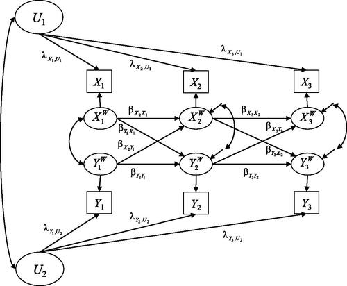
Figure 6. Path diagram of the fixed effects dynamic panel model (FED; Allison et al., 2017) for three measurement waves.

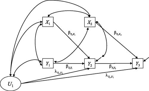
Figure 7. Four different simulation scenarios for a cross-lagged panel design with three measurement waves. Scenario A: true model is a cross-lagged panel model with lag-2 effects (CL2). Scenario B: true model is an observation-level model with a single latent variable (OL1). Scenario C: true model is a residual-level model. Scenario D: true model is a fixed effects dynamic panel model (FED).

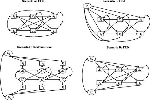
Table 2. Results for Scenario A: True model is the cross-lagged panel model with lag-2 effects (CL2). Estimates of the cross-lagged effect for the different approaches.

Dataset	${\mathrm{\beta }}_{Y_3{X}_1}$	${\mathrm{\beta }}_{Y_3{Y}_1}$	${\mathrm{\beta }}_{Y_3{X}_2}$	CL1	CL2	OL1	OL2	OL3	OL4	RL1	RL2	RL3	FED
A1	0.08	0.27	0.10	0.20	0.10	0.23	0.02	0.01	0.00	0.02	0.02	0.02	0.02
A2	0.01	0.32	0.10	0.20	0.10	0.20	0.05	−0.02	0.14	−0.02	0.22	−0.04	0.18
A3	0.04	0.29	0.12	0.20	0.12	0.23	0.08	0.04	0.00	0.08	0.08	0.08	0.08
A4	−0.01	0.33	0.12	0.20	0.12	0.19	0.11	−0.01	0.15	0.04	0.26	0.03	0.23
A5	0.03	0.27	0.14	0.20	0.14	0.14	0.14	0.08	0.15	0.15	0.25	0.13	0.05
A6	0.00	0.30	0.14	0.20	0.14	0.10	0.14	0.06	0.00	0.14	0.14	0.14	0.14

Note. CL1 = cross-lagged panel model with lag-1 effects; CL2 = cross-lagged panel model with lag-2 effects; OL1 = observation-level model with a single latent factor; OL2 = observation-level model with two latent variables and freely estimated correlations at time 1; OL3 = observation-level model with two latent variables and diagonal loading matrix at time 1; OL4 = OL3 with non-invariant loadings across time; RL1 = residual-level model with diagonal and time-invariant loading matrices and time-invariant regression coefficients; RL2 = RL1 with non-invariant loading matrices; RL3 = RL1 with freely estimated regression coefficients; FED = fixed effects dynamic panel model. ${\mathrm{\beta }}_{Y_3{X}_1}$ = true lag-2 cross-lagged effect of $X_1$ on $Y_3;$ ${\mathrm{\beta }}_{Y_3{Y}_1}$= true lag-2 autoregressive effect of $Y_1$ on $Y_3;$ ${\mathrm{\beta }}_{Y_3{X}_2}$ = true lag-1 cross-lagged effect of $X_2$ on $Y_3.$ Absolute biases for the estimates of the lag-1 cross-lagged effect larger than .02 are printed in bold.

Table 3. Results for Scenario B: True model is the observation-level model with single latent variable (OL1). Estimates of the cross-lagged effect for the different approaches.

Dataset	${\mathrm{\rho }}_{Y_1{U}_1}$	${\mathrm{\rho }}_{Y_2{U}_1}$	${\mathrm{\rho }}_{Y_3{U}_1}$	${\mathrm{\rho }}_{X_1{U}_1}$	${\mathrm{\rho }}_{X_2{U}_1}$	${\mathrm{\rho }}_{X_3{U}_1}$	${\mathrm{\beta }}_{Y_3{X}_2}$	CL1	CL2	OL1	OL2	OL3	OL4	RL1	RL2	RL3	FED
B1	0.50	0.50	0.50	0.30	0.30	0.30	0.20	0.21	0.20	0.20	0.20	0.20	0.20	0.20	0.20	0.20	0.20
B2	0.50	0.50	0.50	0.30	0.15	0.08	0.20	0.17	0.16	0.21	0.19	0.18	0.18	0.19	0.21	0.17	0.18
B3	0.50	0.25	0.13	0.30	0.15	0.08	0.20	0.20	0.20	0.20	0.17	0.18	0.20	0.20	0.15	0.20	0.19
B4	0.50	0.25	0.13	0.30	0.30	0.30	0.20	0.19	0.19	0.20	0.17	0.19	0.19	0.14	0.20	0.14	0.20
B5	0.05	0.10	0.20	0.30	0.30	0.30	0.20	0.23	0.22	0.20	0.18	0.19	0.20	0.21	0.17	0.22	0.14
B6	0.05	0.15	0.45	0.30	0.30	0.30	0.20	0.29	0.27	0.20	0.16	0.17	0.20	0.21	0.05	0.25	–0.01

Note. CL1 = cross-lagged panel model with lag-1 effects; CL2 = cross-lagged panel model with lag-2 effects; OL1 = observation-level model with a single latent factor; OL2 = observation-level model with two latent variables and freely estimated correlations at time 1; OL3 = observation-level model with two latent variables and diagonal loading matrix at time 1; OL4 = OL3 with non-invariant loadings across time; RL1 = residual-level model with diagonal and time-invariant loading matrices and time-invariant regression coefficients; RL2 = RL1 with non-invariant loading matrices; RL3 = RL1 with freely estimated regression coefficients; FED = fixed effects dynamic panel model. ${\mathrm{\rho }}_{Y_1{U}_1}$= true correlation between $Y_1$ and $U_1;$ ${\mathrm{\rho }}_{Y_2{U}_1}$ = true correlation between $Y_2$ and $U_1;$ ${\mathrm{\rho }}_{Y_3{U}_1}$ = true correlation between $Y_3$ and $U_1;$ ${\mathrm{\rho }}_{X_1{U}_1}$ = true correlation between $X_1$ and $U_1;$ ${\mathrm{\rho }}_{X_2{U}_1}$ = true correlation between $X_2$ and $U_1;$ ${\mathrm{\rho }}_{X_3{U}_1}$ = true correlation between $X_3$ and $U_1;$ ${\mathrm{\beta }}_{Y_3{X}_2}$ = true cross-lagged effect of $X_2$ on $Y_3$ in the data-generating model OL1. Absolute biases for the estimates of the cross-lagged effect larger than .02 are printed in bold.

Table 4. Results for Scenario C: True Model is the residual-level (RL) Model. Estimates for the cross-lagged effect for the different approaches.

Dataset	${\mathrm{\varphi }}_{U_1}$	${\mathrm{\beta }}_{Y_2{X}_1}$	${\mathrm{\lambda }}_{Y_2,U_2}$	${\mathrm{\beta }}_{Y_3{X}_2}$	CL1	CL2	OL1	OL2	OL3	OL4	RL1	RL2	RL3	FED
C1	0.30	0.20	1.00	0.20	0.13	0.17	0.24	0.20	0.15	0.09	0.20	0.20	0.20	0.20
C2	0.50	0.20	1.00	0.20	0.12	0.16	0.27	0.20	0.12	0.02	0.20	0.20	0.20	0.20
C3	0.70	0.20	1.00	0.20	0.11	0.15	0.29	0.20	0.07	−0.02	0.20	0.20	0.20	0.20
C4	0.30	0.05	1.00	0.20	0.13	0.15	0.02	0.00	0.10	0.02	0.11	0.04	0.19	−0.10
C5	0.50	0.05	1.00	0.20	0.12	0.15	0.15	0.01	0.07	0.04	0.12	0.03	0.19	−0.10
C6	0.70	0.05	1.00	0.20	0.11	0.13	0.23	0.05	0.03	0.05	0.12	0.18	0.19	−0.10
C7	0.30	0.20	0.80	0.20	0.13	0.16	0.16	0.19	0.18	0.16	0.20	0.20	0.20	0.17
C8	0.50	0.20	0.80	0.20	0.13	0.15	0.11	0.17	0.16	0.09	0.22	0.20	0.22	0.14
C9	0.70	0.20	0.80	0.20	0.12	0.14	0.07	0.14	0.13	0.03	0.25	0.20	0.25	0.10

Note. CL1 = cross-lagged panel model with lag-1 effects; CL2 = cross-lagged panel model with lag-2 effects; OL1 = observation-level model with a single latent factor; OL2 = observation-level model with two latent variables and freely estimated correlations at time 1; OL3 = observation-level model with two latent variables and diagonal loading matrix at time 1; OL4 = OL3 with non-invariant loadings across time; RL1 = residual-level model with diagonal and time-invariant loading matrices and time-invariant regression coefficients; RL2 = RL1 with non-invariant loading matrices; RL3 = RL1 with freely estimated regression coefficients; FED = fixed effects dynamic panel model. ${\mathrm{\varphi }}_{U_1}$= Variance of $U_1;$ ${\mathrm{\beta }}_{Y_2{X}_1}$ = true lag-1 cross-lagged effect of $X_1$ on $Y_2;$ ${\mathrm{\lambda }}_{Y_2,U_2}$= loading of $Y_2$ on $U_2$ (0.80 indicates that loadings are noninvariant across time); ${\mathrm{\beta }}_{Y_3{X}_2}$ = true lag-1 cross-lagged effect of $X_2$ on $Y_3$ in the residual-level model. Absolute biases for the estimates of the lag-1 cross-lagged effect larger than .02 are printed in bold.

Table 5. Results for Scenario D: True model is the fixed effects dynamic panel model (FED). Estimates for the cross-lagged effect for the different approaches.

Dataset	${\mathrm{\varphi }}_{U_1}$	${\mathrm{\lambda }}_{X_3,U_1}$	${\mathrm{\beta }}_{X_3{Y}_1}$	${\mathrm{\beta }}_{Y_3{X}_2}$	CL1	CL2	OL1	OL2	OL3	OL4	RL1	RL2	RL3	FED
D1	0.5	0.5	0	0.20	0.21	0.23	0.20	0.20	0.20	0.20	0.27	0.27	0.27	0.20
D2	0.7	0.5	0	0.20	0.25	0.29	0.27	0.20	0.20	0.19	0.39	0.17	0.41	0.20
D3	0.5	0.15	0	0.20	0.21	0.23	0.19	0.22	0.23	0.20	0.26	0.30	0.26	0.20
D4	0.7	0.15	0	0.20	0.25	0.29	0.24	0.25	0.27	0.20	0.32	0.38	0.32	0.20
D5	0.5	0.5	0.07	0.20	0.21	0.23	0.22	0.09	0.14	0.15	0.19	0.08	0.22	0.20
D6	0.7	0.5	0.07	0.20	0.25	0.29	0.24	−0.03	0.08	0.12	−0.02	0.00	0.33	0.20
D7	0.5	0.15	0.07	0.20	0.21	0.23	−0.41	0.20	0.20	0.23	0.22	0.25	0.22	0.20
D8	0.7	0.15	0.07	0.20	0.25	0.29	0.43	0.23	0.26	0.25	0.28	0.34	0.28	0.20

Note. CL1 = cross-lagged panel model with lag-1 effects; CL2 = cross-lagged panel model with lag-2 effects; OL1 = observation-level model with a single latent factor; OL2 = observation-level model with two latent variables and freely estimated correlations at time 1; OL3 = observation-level model with two latent variables and diagonal loading matrix at time 1; OL4 = OL3 with non-invariant loadings across time; RL1 = residual-level model with diagonal and time-invariant loading matrices and time-invariant regression coefficients; RL2 = RL1 with non-invariant loading matrices; RL3 = RL1 with freely estimated regression coefficients; FED = fixed effects dynamic panel model. ${\mathrm{\varphi }}_{U_1}$= Variance of $U_1;$ ${\mathrm{\lambda }}_{X_3,U_1}$= loading of $X_3$ on $U_1$ (0.15 indicates that loadings are noninvariant across time); ${\mathrm{\beta }}_{X_3{Y}_1}$= true lag-2 cross-lagged effect of $Y_1$ on $X_3;$ ${\mathrm{\beta }}_{Y_3{X}_2}$ = true lag-1 cross-lagged effect of $X_2$ on $Y_3$ in the fixed effects dynamic panel model FED. Absolute biases for the estimates of the lag-1 cross-lagged effect larger than .02 are printed in bold.

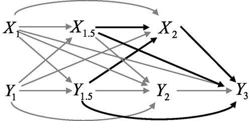
Figure 8. Process of X_t and Y_t considered at time points 1, 2, 2.5, and 3 (upper panel), and time points 1, 2, 2.33, 2.67, and 3 (lower panel). Thick paths are included in the causal cross-lagged effect of X₂ on Y₃ (with adjustment for X₁, Y₁, and Y₂).

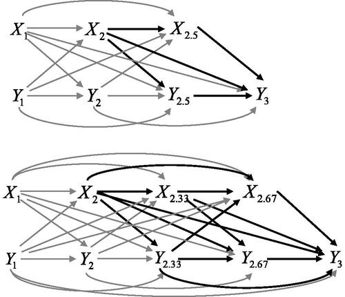
Figure 9. Process of X_t and Y_t considered at time points 1, 1.5, 2, and 3. Thick paths are included in the causal cross-lagged effect of X₂ on Y₃ (with adjustment for X₁, Y₁, and Y₂).

Finkel, S. (1995). Causal analysis with panel data. Sage. http://dx.doi.org/10.4135/9781412983594

 Google Scholar

Dishop, C. R., & DeShon, R. P. (2021). A tutorial on Bollen and Brand’s approach to modeling dynamics while attending to dynamic panel bias. Psychological Methods, Advance online publication. https://doi.org/10.1037/met0000333

 Google Scholar

Bollen, K. A., & Brand, J. E. (2010). A general panel model with random and fixed effects: A structural equations approach. Social Forces, 89, 1–34. https://doi.org/10.1353/sof.2010.0072

 PubMed Web of Science ®Google Scholar

Zyphur, M. J., Allison, P. D., Tay, L., Voelkle, M. C., Preacher, K. J., Zhang, Z., Hamaker, E. L., Shamsollahi, A., Pierides, D. C., Koval, P., & Diener, E. (2020). From data to causes I: Building a general cross-lagged panel model (GCLM). Organizational Research Methods, 23, 651–687. http://dx.doi.org/10.1177/1094428119847278

 Web of Science ®Google Scholar

Hamaker, E. L., Kuiper, R. M., & Grasman, R. P. P. P. (2015). A critique of the cross-lagged panel model. Psychological Methods, 20, 102–116. http://dx.doi.org/10.1037/a0038889

 PubMed Web of Science ®Google Scholar

Allison, P. D., Williams, R., & Moral-Benito, E. (2017). Maximum likelihood for cross-lagged panel models with fixed effects. Socius, 3, 237802311771057. https://doi.org/10.1177/2378023117710578

 Google Scholar