An Alternative Prior for Estimation in High-Dimensional Settings

Figures & data

Figure 1. Marginal density of the Dirichlet-horseshoe (DHS) in comparison with those of the double exponential (DE), horseshoe (HS), Dirichlet-Laplace (DL), and regularized horseshoe (RHS) priors.

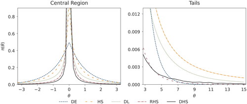
Figure 2. Squared error loss corresponding to the posterior median derived from the normal means problem (Simulation Study I), with a D = 400 dimensional parameter vector for varying signal strengths $A\in \{4,5,6\}$ and sparsity ratios $q_D=5\%$ (left panel) and $q_D=10\%$ (right panel). We abbreviate the considered priors SPSL (spike-and-slab), BAL (Bayesian Adaptive lasso), HS (horseshoe), DL (Dirichlet-Laplace), RHS (regularized horseshoe), and DHS (Dirichlet-horseshoe).

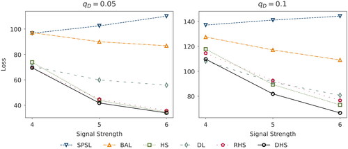
Figure 3. Squared error loss corresponding to the posterior median for different hyperparameter choices ν, derived from the normal means problem with a D = 400 dimensional parameter vector, sparsity ratio $q_D=5\%,$ and varying signal strengths $A\in \{4,5,6\}.$

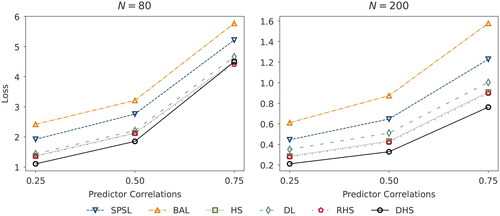
Figure 4. Squared error loss corresponding to the posterior median derived from the multiple regression setting (Simulation Study II) with a D = 100 dimensional parameter vector drawn from a log-normal distribution for varying correlations $\rho \in \{0.25,0.5,0.75\}$ and observations N = 80 (left panel) and N = 200 (right panel). The design matrix is generated by a multivariate normal distribution with correlated predictors. The parameter vector $\mathit{\beta }$ has a sparsity ratio of 20%, such that we set 80 of the 100 predictors to 0. We abbreviate the priors SPSL (spike-and-slab), BAL (Bayesian Adaptive lasso), HS (horseshoe), DL (Dirichlet-Laplace), RHS (regularized horseshoe), and DHS (Dirichlet-horseshoe).

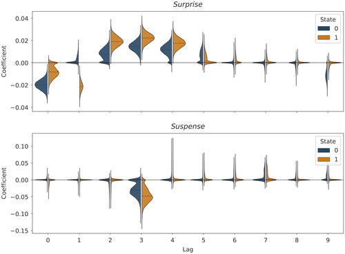
Figure 5. Posterior distributions of the effects of the emotional cues Surprise and Suspense on beer sales, derived from the real-data example. The figure shows posteriors for all lags in both states (negative S = 0 and positive S = 1). The dotted lines indicate the estimated median effect.

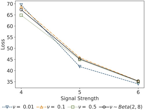
Table 1. This table provides a brief summary of the properties of prior distributions.

Spike-and-Slab	Bayesian (Adaptive) Lasso
discrete (point-mass mixture) prior; continuous versions exist	continuous shrinkage prior
good performance in most settings, in terms of sparsity	simple and fast computations
well-understood theoretical properties	ensures unimodal posteriors
computationally intensive in high-dimensional spaces	limited flexibility and adaptivity
results sensitive to hyperprior choices difficulties in modeling correlated predictors difficulties in modeling class variables with more than two levels	undershrinkage of noise and overshrinkage of large coefficients overestimation of signal density
Horseshoe	Dirichlet-Laplace
continuous shrinkage prior	continuous shrinkage prior
good performance in high-dimensional, sparse settings	existing closed-form representation
adaptivity to unknown sparsity and signal-to-noise ratio	efficient posterior computation
complexity not dependent on number of observations	optimal posterior concentration
no possibility of including prior knowledge of sparsity ratios over- and underestimation of sparsity ratio large coefficients left unshrunk correlated predictors can cause multimodal posteriors convergence and sampling issues	results strongly dependent on unknown concentration parameter
Regularized Horseshoe
continuous shrinkage prior	generalization of the horseshoe that nests it
good performance in high-dimensional settings improved sampling robustness results sensitive to hyperparameter choices	ability to include prior knowledge about the degree of sparsity correlated predictors can cause multimodal posteriors

Table A1. This table presents performance metrics based on 95% HDIs, averaged across simulation replicates. The measures are derived from the normal means problem (Simulation Study I) with a D = 400 dimensional parameter vector. We perform Ω = 100 replications for all combinations of signals strengths $A\in \{4,5,6\}$ and sparsity ratios $q_D\in \{0.05,0.1\}.$ We consider the spike-and-slab (SPSL), Bayesian Adaptive lasso (BAL), horseshoe (HS), Dirichlet-Laplace (DL), regularized horseshoe (RHS), and Dirichlet-horseshoe (DHS) priors.

		Loss	StdLoss	StdMedian	Coverage	Loss	StdLoss	StdMedian	Coverage
A = 4	SPSL	96.6	0.1431	0.6510	0.9812	137.0	0.1348	0.7284	0.9747
	BAL	97.1	0.1689	0.7146	0.9923	127.0	0.1496	0.7334	0.9857
	HS	73.8	0.2784	0.4539	0.9892	118.0	0.1957	0.5862	0.9815
	DL	70.6	0.2244	0.6309	0.9919	108.0	0.1840	0.6546	0.9845
	RHS	69.3	0.2673	0.5014	0.9889	114.0	0.1822	0.6330	0.9814
	DHS	69.5	0.2939	0.4494	0.9900	110.0	0.2057	0.5875	0.9826
A = 5	SPSL	102.0	0.1411	0.6951	0.9852	141.0	0.1273	0.7587	0.9859
	BAL	90.0	0.1739	0.7137	0.9955	117.0	0.1581	0.7310	0.9913
	HS	43.9	0.3480	0.4728	0.9935	89.4	0.2312	0.5997	0.9889
	DL	59.9	0.2387	0.6292	0.9956	91.3	0.2032	0.6510	0.9909
	RHS	44.8	0.3369	0.5020	0.9931	92.6	0.2126	0.6310	0.9905
	DHS	41.8	0.3582	0.4535	0.9938	81.9	0.2471	0.5772	0.9893
A = 6	SPSL	110.0	0.1436	0.7243	0.9878	144.0	0.1187	0.7788	0.9871
	BAL	86.8	0.1711	0.7128	0.9957	109.0	0.1431	0.7295	0.9922
	HS	34.6	0.3198	0.4743	0.9971	73.1	0.1925	0.6025	0.9927
	DL	55.8	0.2292	0.6277	0.9962	80.8	0.1732	0.6490	0.9922
	RHS	35.8	0.3181	0.4934	0.9968	76.7	0.1892	0.6239	0.9925
	DHS	34.0	0.3303	0.4470	0.9971	66.7	0.2099	0.5653	0.9931

Table A2. See the descriptive notes to Table A1.

		TypeIErr	Rhat	Minutes	Divergences	TypeIErr	Rhat	Minutes	Divergences
A = 4	SPSL	0.0004	1.00	0.4216	0	0.0012	1	0.4864	0
	BAL	0.0012	1.00	2.00	21	0.0015	1.00	1.90	31
	HS	0.0001	1.00	0.9389	118	0.0002	1.00	1.11	105
	DL	0.0005	1.00	2.54	0	0.0005	1.00	2.42	0
	RHS	0.0001	1.00	0.4583	0	0.0005	1	0.4244	0
	DHS	0.0001	1.00	4.68	7.49	0.0003	1.00	4.29	3.38
A = 5	SPSL	0.0009	1.00	0.5204	0	0.0017	1	0.4934	0
	BAL	0.0014	1.00	1.97	25.4	0.0012	1.00	1.88	30.9
	HS	0.0001	1.00	0.9861	131	0.0003	1.00	1.34	95
	DL	0.0006	1.00	2.40	0	0.0006	1.00	2.42	0
	RHS	0.0001	1.00	0.4315	0.0400	0.0005	1	0.4438	0
	DHS	0.0002	1.01	4.47	4.60	0.0003	1.00	4.44	1.83
A = 6	SPSL	0.0014	1.00	0.4924	0	0.0024	1	0.5030	0
	BAL	0.0014	1.00	1.89	23	0.0013	1.00	1.88	31.8
	HS	0.0001	1.00	1.09	116	0.0003	1.00	1.36	109
	DL	0.0005	1.00	2.42	0	0.0005	1.00	2.41	0
	RHS	0.0002	1.00	0.4359	0	0.0005	1	0.4540	0
	DHS	0.0001	1.00	4.45	1.40	0.0003	1.00	4.47	1.25

Table A3. This table presents performance metrics based on 95% HDIs, averaged across simulation replicates. The measures are derived from the multiple regression setting (Simulation Study II) with a D = 100 dimensional parameter vector drawn from a log-normal distribution. The design matrix is generated by a multivariate normal distribution with correlated predictors. We perform Ω = 100 replications for all combinations of observations $N\in \{80,200\}$ and correlations $\rho \in \{0.25,0.5,0.75\}.$ We consider the spike-and-slab (SPSL), Bayesian Adaptive lasso (BAL), horseshoe (HS), Dirichlet-Laplace (DL), regularized horseshoe (RHS), and Dirichlet-horseshoe (DHS) priors.

		Loss	StdLoss	StdMedian	Coverage	Loss	StdLoss	StdMedian	Coverage
\rho = 0.25	SPSL	1.92	0.4223	0.2256	0.9948	0.4456	0.2645	0.0869	0.9885
	BAL	2.42	0.4099	0.2744	0.9972	0.6116	0.2233	0.0946	0.9841
	HS	1.37	0.4449	0.1579	0.9878	0.2860	0.3186	0.0721	0.9884
	DL	1.44	0.4377	0.1917	0.9939	0.3525	0.2883	0.0804	0.9898
	RHS	1.35	0.4422	0.1586	0.9884	0.2791	0.3235	0.0715	0.9879
	DHS	1.11	0.5348	0.1280	0.9868	0.2121	0.3872	0.0594	0.9881
\rho = 0.50	SPSL	2.76	0.3267	0.2600	0.9946	0.6471	0.2536	0.1057	0.9898
	BAL	3.21	0.2827	0.3114	0.9981	0.8737	0.2278	0.1144	0.9870
	HS	2.13	0.3693	0.1903	0.9864	0.4316	0.2859	0.0879	0.9887
	DL	2.21	0.3544	0.2291	0.9939	0.5116	0.2752	0.0977	0.9907
	RHS	2.12	0.3599	0.1944	0.9868	0.4198	0.2910	0.0868	0.9885
	DHS	1.85	0.4337	0.1624	0.9850	0.3291	0.3506	0.0741	0.9888
\rho = 0.75	SPSL	5.22	0.3433	0.3254	0.9904	1.23	0.2698	0.1467	0.9885
	BAL	5.77	0.3284	0.3875	0.9954	1.58	0.2455	0.1574	0.9866
	HS	4.50	0.3840	0.2512	0.9805	0.9078	0.2818	0.1221	0.9860
	DL	4.66	0.4054	0.3030	0.9903	1.00	0.2915	0.1356	0.9884
	RHS	4.41	0.3748	0.2590	0.9826	0.8957	0.2844	0.1216	0.9856
	DHS	4.49	0.4476	0.2254	0.9768	0.7623	0.3345	0.1064	0.9857

Table A4. See the descriptions for Table A3.

		TypeIErr	Rhat	Minutes	Divergences	TypeIErr	Rhat	Minutes	Divergences
\rho = 0.25	SPSL	0.0000	1.00	0.3974	0	0.0025	1.00	0.5614	0
	BAL	0.0000	1.00	0.8220	120	0.0076	1.00	0.9750	94.5
	HS	0.0003	1.00	0.7104	64.9	0.0005	1.00	0.9305	76.8
	DL	0.0001	1.00	0.9277	0.3800	0.0014	1.00	1.06	2.99
	RHS	0.0003	1.00	0.5096	0.1500	0.0005	1.01	0.6999	0.4700
	DHS	0.0003	1.00	1.58	11	0.0003	1.01	1.66	24.7
\rho = 0.50	SPSL	0.0004	1.00	0.5328	0	0.0022	1.00	0.6584	0
	BAL	0.0001	1.00	0.8209	82.4	0.0063	1.00	0.9727	79.8
	HS	0.0003	1.00	0.7402	69.1	0.0006	1.00	0.9357	58.6
	DL	0.0001	1.00	0.9274	1.17	0.0011	1.00	1.06	6.06
	RHS	0.0003	1.01	0.5613	0.0700	0.0005	1.00	0.9318	0.3900
	DHS	0.0001	1.00	1.58	13.4	0.0003	1.00	1.66	23
\rho = 0.75	SPSL	0.0006	1.00	0.6019	0	0.0022	1.00	0.8126	0
	BAL	0.0004	1.00	0.8207	68.8	0.0046	1.00	0.9755	88
	HS	0.0006	1.00	0.7695	71.2	0.0004	1.00	0.9376	79.6
	DL	0.0006	1.00	0.9262	1.36	0.0013	1.00	1.06	6.39
	RHS	0.0009	1.00	0.6668	0.0400	0.0006	1.00	1.07	0.1300
	DHS	0.0009	1.00	1.58	10.5	0.0004	1.00	1.66	16.3

Data Availability Statement

The data and code that support the findings of this study are openly available at https://zenodo.org/doi/10.5281/zenodo.10707994.