Causal Effects of Time-Varying Exposures: A Comparison of Structural Equation Modeling and Marginal Structural Models in Cross-Lagged Panel Research

Figures & data

Table 1. Glossary of causal inference-related terms used in this article.

Term	Description and related terms
Exposure regime	A rule that determines the value of a time-varying exposure for each time point (Hernán & Robins, 2020). In case of a dichotomous exposure variable, an exposure regime is thus a specific sequence of 0’s and 1’s, indicating for each time point whether treatment or no treatment is given. Here, we discuss static regimes, implying that exposure values are all predetermined. Related term: exposure sequence.
Always-exposed	An exposure regime in which a binary exposure is set to “exposed” for all predefined number of time points.
Never-exposed	An exposure regime in which a binary exposure is set to “not exposed” for all predefined number of time points.
Causal estimand	A precise description of an effect, reflecting the research question of a research project. It summarizes at a population-level what the outcomes would be in the same individuals under different exposure conditions (European Medicines Agency, 2020). Causal estimands are often defined as functions (e.g., contrasts) of potential outcomes. Related term: target causal quantity (Petersen & Van der Laan, 2014).
Causal identification	The process of translating a causal estimand to a statistical estimand, which is defined as a function of observed data. It involves evaluation of the causal identification assumptions of exchangeability, consistency, and positivity.
Exchangeability	A causal identification assumption restricting the exposure to be independent from the potential outcomes (Angrist & Pischke, 2009; Hernán & Robins, 2020; Imbens & Rubin, 2015). Violated in settings with confounding/selection bias. Related terms: unconfounded assignment, unconfoundedness, no unmeasured confounding, (conditional) independence of treatment and potential outcomes, exogeneity (Rosenbaum & Rubin, 1983).
Consistency	A causal identification assumption linking potential outcomes to observed outcomes. It is violated when exposure is not well-defined and/or there exist multiple versions of intervention/treatment (Hernán, 2016).
Causal directed acyclical graphs (DAGs)	A diagram, consisting of nodes and edges connecting them, visualizing a data generating process. Nodes represent variables in the phenomenon under study, and edges the causal relationships between them. All variables thought to play a role in the causal process should be included. Related terms: causal diagrams, non-parametric structural equation model (Pearl, 2009)

Figure 1. A simplified representation of the causal DAG relating smoking cessation and body weight. It includes the variables smoking cessation, body weight, baseline covariates, and time-varying covariates. The arrows represent the nonparametric links between them. ${}^{‡}$Age, sex, ethnicity. ${}^{*}$Body weight, socioeconomic factors, alcohol consumption, physical activity, energy intake, and comorbidities.

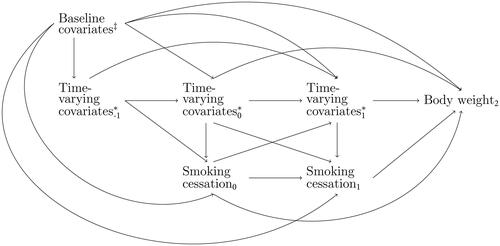
Table 2. Overview of covariates included in the LISS panel study.

Covariate	Measurement level	Measurement time	Time-span
Age	Continuous	Baseline	Right now
Sex	Nominal	Baseline	Right now
Body weight	Continuous	Time-varying	Right now
Alcohol consumption	Ordinal	Time-varying	Average last year
Hours physical activity	Continuous	Time-varying	Average last week
Number of comorbidities^a	Ordinal	Time-varying	Last year

Note. All variables are self-reported measures taken from a questionnaire.

^a Self reported information on diagnosis by a physician.

Figure 2. Density of propensity scores for individuals who quit smoking versus individuals who continued smoking at time points 0 and 1 (before weighting). Propensity scores were computed using all covariates.

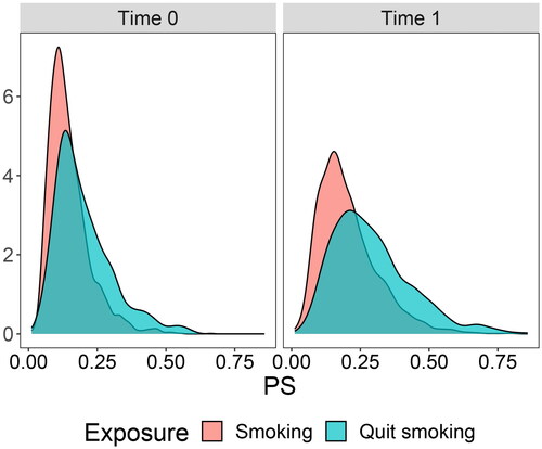
Figure 3. Visualization of covariate balance (standardized mean differences) before and after reweighing at time points 0 and 1. The asterisk * denotes binary covariates (or dummy variables) for which the displayed value is the raw (unstandardized) difference in means. PW = per week; PM = per month; P2M = per two months; PY = per year.

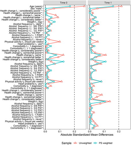
Figure 4. The causal structure of the data generating mechanisms used in the simulations.

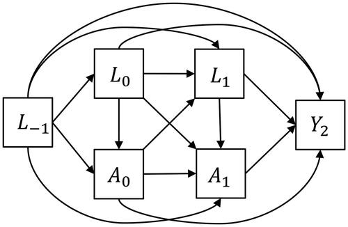
Figure 5. Overview of data generating mechanisms (DGMs) 2, 3, and 4. Bold black arrows in the DAGs indicate nonlinear dependencies. These direct effects are visualized in the plots to the right of each respective DGM, with the solid black line representing the true (nonlinear) functional relationship between two variables, and the dashed blue line representing the linear projection. DGM 1 (not illustrated here) contains only linear dependencies. DGM 5 (not illustrated here) combines the nonlinear dependencies of DGMs 2, 3, and 4.

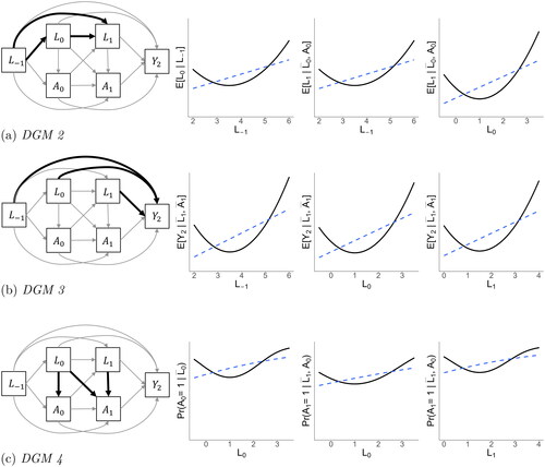
Figure 6. Bias in the point estimates of the always-exposed versus never-exposed effect across five methods: “IPW (L)” is linear IPW regression; “path (L) is linear path analysis; “IPW (L, Q)” is IPW regression with linear and quadratic terms in DGMs 3, 4, and 5; “path (L, Q)” is path analysis with linear and quadratic terms in DGMs 2, 3, 4, and 5; “unadjusted” is a linear regression without confounding adjustment. Results are presented for the case of n = 1,000, 10% and 50% exposed, and across five DGMs.

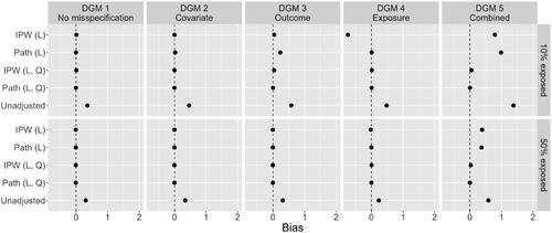
Figure 7. MSE of the point estimates of the always-exposed versus never-exposed effect across five methods, and five DGMS (n = 1,000).

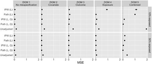
Table A1. Population values used for data generation.

Causal effect	Population value
$L_{-1}\to \dots$	0.1^a
$L_0\to A_0$	0.5
$L_0\to L_1$	0.3
$L_0\to A_1$	0.25
$L_0\to Y_2$	0.15
$A_0\to L_1$	0.4
$A_0\to A_1$	0.8
$A_0\to Y_2$	0.2
$L_1\to A_1$	0.5
$L_1\to Y_2$	0.3
$A_1\to Y_2$	0.4

^a This value applies to all effects of $L_{-1}.$

Hernán, M. A., & Robins, J. M. (2020). Causal inference: What if. Chapman & Hall/CRC.

 Google Scholar

European Medicines Agency. (2020). ICH E9 (R1) addendum on estimands and sensitivity analysis in clinical trials to the guideline on statistical principles for clinical trials. https://www.ema.europa.eu/en/documents/scientific-guideline/ich-e9-r1-addendum-estimands-sensitivity-analysis-clinical-trials-guideline-statistical-principles_en.pdf

 Google Scholar

Petersen, M. L., & Van der Laan, M. J. (2014). Causal models and learning from data: Integrating causal modeling and statistical estimation. Epidemiology, 25, 418–426. https://doi.org/10.1097/EDE.0000000000000078

 PubMed Web of Science ®Google Scholar

Angrist, J. D., & Pischke, J.-S. (2009). Mostly harmless econometrics: An empiricist’s companion. Princeton University Press. https://doi.org/10.1515/9781400829828

 Google Scholar

Imbens, G. W., & Rubin, D. B. (2015). Causal inference for statistics, social, and biomedical sciences: An introduction (1st ed.). Cambridge University Press. https://doi.org/10.1017/CBO9781139025751

 Google Scholar

Rosenbaum, P. R., & Rubin, D. B. (1983). The central role of the propensity score in observational studies for causal effects. Biometrika, 70, 41–55. https://doi.org/10.1093/biomet/70.1.41

 Web of Science ®Google Scholar

Hernán, M. A. (2016). Does water kill? A call for less casual causal inferences. Annals of Epidemiology, 26, 674–680. https://doi.org/10.1016/j.annepidem.2016.08.016

 PubMed Web of Science ®Google Scholar

Pearl, J. (2009). Causality: Models, reasoning, and inference (2nd ed.). Cambridge University Press. https://doi.org/10.1017/CBO9780511803161

 Google Scholar