Health and lifespan of Swiss men born in an alpine region in 1905–1907

Figures & data

Figure 1. A) Topographical map of the Canton of Glarus(source: www.geo.gl.ch). B) Municipalities, regions, and share of industrial workers in 1920. The polygons represent the 29 municipalities coloured in grey scales according to the four main regions (Lower Main Valley, Upper Main Valley, Linthal valley, and Sernftal valley). The circles represent the main places of the municipalities, and their size is proportional to the population size in the 1920 census (min = 219, max = 5027). The colours of the circles indicate the share of industrial workers (in tertiles) in 1920.

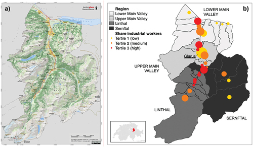
Table 1. Descriptive statistics categorical variables. A) Full sample; B) Only citizens of the Canton of Glarus (GL) (as only these people can be linked to the genealogical register).

	A) Full sample					B) GL citizens only
	Variable	N	%	Mean height	SD	Variable	N	%	Mean height	SD
Place of citizenship	Lower main valley	278	25.9	166.24	6.72	Lower main valley	278	33.6	166.24	6.72
	Upper main valley	246	22.9	168.43	6.46	Upper main valley	246	29.7	168.43	6.46
	Linthal	120	11.2	169.14	6.99	Linthal	120	14.5	169.14	6.99
	Sernftal	183	17.1	167.66	6.55	Sernftal	183	22.1	167.66	6.55
	Outside GL	246	22.9	167.41	6.83
	Total	1073	100.0			Total	827	100.0
HISCLASS	Unskilled workers	236	22.3	165.10	7.23	Unskilled workers	172	21.2	165.01	7.26
	Skilled workers	431	40.8	167.74	6.26	Skilled workers	293	36.1	167.62	6.13
	Farmers	197	18.6	167.16	6.02	Farmers	178	21.9	167.28	6.01
	Lower middle class	132	12.5	170.45	6.69	Lower middle class	117	14.4	170.56	6.74
	Elite	61	5.8	171.13	6.38	Elite	51	6.3	170.98	6.33
	Total	1057	100.0			Total	811	100.0
Region of residence	Lower main valley	228	21.2	166.35	6.78	Lower main valley	174	21.0	166.06	6.47
	Upper main valley	254	23.7	168.32	6.70	Upper main valley	159	19.2	168.54	6.48
	Linthal	136	12.7	166.79	6.58	Linthal	82	9.9	167.05	6.97
	Sernftal	134	12.5	167.67	6.44	Sernftal	105	12.7	167.81	6.39
	Outside GL	321	29.9	168.16	6.84	Outside GL	307	37.1	168.13	6.91
	Total	1073	100.0			Total	827	100.0
Fitness to serve	Fit	669	63.3	168.04	5.94	Fit	522	63.8	168.16	5.97
	Deferred	127	12.0	168.28	7.35	Deferred	101	12.3	168.41	7.23
	Auxiliary service	152	14.4	167.01	7.20	Auxiliary service	119	14.5	167.03	7.15
	Unfit	109	10.3	164.50	9.14	Unfit	76	9.3	163.82	8.91
	Total	1057	100.0			Total	818	100.0
Age (y)	19/20	992	92.5	167.41	6.70	19/20	762	92.3	167.46	6.71
	≥21	80	7.5	169.74	6.98	≥21	64	7.7	169.70	6.66
	Total	1072	100.0			Total	826	100.0
Goitre status	No goitre	693	64.6	167.33	6.95	No goitre	568	68.7	167.53	7.00
	goitre	380	35.4	168.03	6.34	goitre	259	31.3	167.85	6.07
	Total	1073	100.0			Total	827	100.0
BMI est. (kg/m^2)	<18.5	28	2.6	163.25	9.13	<18.5	19	2.3	163.16	8.36
	18.5–24.9	1020	95.1	167.69	6.64	18.5–24.9	786	95.0	167.73	6.64
	25.0–29.9	25	2.3	167.80	6.80	25.0–29.9	22	2.7	167.77	7.09
	Total	1073	100.0			Total	827	100.0

Table 2. Descriptive statistics numerical variables (histograms displayed in Appendix Figure S3). GL = Canton of Glarus.

Continuous variable	Data	N	Mean	SD	Min	Max
Height (cm)	Full sample	1073	167.58	6.75	138	189
	GL citizens	827	167.63	6.72	138	189
Chest circumference (cm)	Full sample	1073	86.46	4.92	67	105
	GL citizens	827	86.47	4.96	70	101
Upper arm circumference (cm)	Full sample	1073	25.86	1.94	18	36
	GL citizens	827	25.84	1.94	18	36
BMI est. (kg/m^2)	Full sample	1073	21.76	1.63	16.64	27.45
	GL citizens	827	21.74	1.64	16.64	27.45
Age (y)	Full sample	1072	20.13	0.65	18	32
	GL citizens	826	20.14	0.70	18	32
Lifespan (y)	GL citizens	635	72.62	14.36	22.7	102.15
Cohort life expectancy at age 20 (y)	GL citizens	635	55.01	17.32	2.7	82.15

Figure 2. Coefficient plots visualising the results of the OLS regressions explaining A) mean height and B) mean estimated BMI. The error bars indicate 95% confidence intervals. GL = Canton of Glarus. Full results: See Appendix. Table S2

Figure 3. Kaplan Meier curves for survival probabilities showing the results of the multivariable Cox proportional hazards regression models for categorised height (A) and estimated BMI (B). Full results are presented in Appendix. Table S3

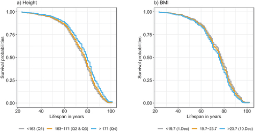
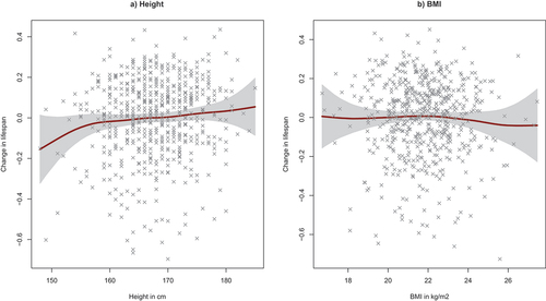
Figure 4. Results from the GAM models explaining variance in lifespan. Only the effect of the smoothed terms height (A) and estimated BMI (B) are shown in the plots, the full results (including HISCLASS, region, fitness to serve, age, and goitre status) can be found in Appendix Table S4. Grey areas indicate 95% confidence intervals.