Medium range sea ice prediction in support of Japanese research vessel MIRAI’s expedition cruise in 2018

Figures & data

Figure 1. Cruise tracks of the research vessel MIRAI in 2018 and locations for conductivity, temperature and depth (CTD) observations. Vertical profiles along track A–B are shown in Figure 7.

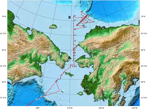
Figure 2. Bathymetry (m) of (a) Pan-Arctic model domain, and (b) high-resolution regional model domain, which includes the Chukchi Sea and Bering Strait. Red rectangle in (a) indicates the location of (b).

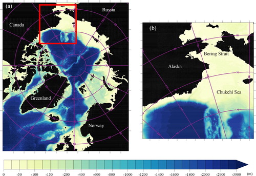
Figure 3. Schematic diagram of predicted (blue) and observational (red) ice edges. Yellow areas indicate model overestimation (O), which is the spatial integral of all sea ice extents where predicted ice concentration is above 15% but observed ice concentration is below 15%. Green areas indicate model underestimation (U), which is the spatial integral of all sea ice extents where predicted ice concentration is below 15% but observed ice concentration is above 15%. Light blue and white areas indicate ocean extent that has been correctly predicted and sea ice extent that has been correctly predicted, respectively.

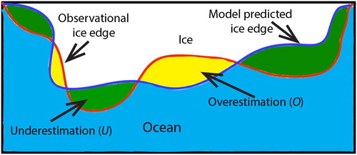
Figure 4. Evolution of difference between predicted and Advanced Microwave Scanning Radiometer 2 (AMSR2) observational sea ice concentration distributions for 9–19 November 2018. Model run starts from 9 November 2018. Black contour indicates AMSR2 ice edge (15% concentration threshold). Green dots indicate locations of ice edge observed from MIRAI. Aerial photos taken from the same locations are shown in Figure 5.

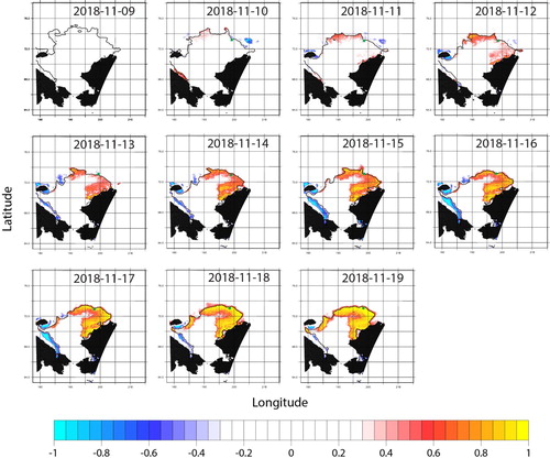
Figure 5. Sea ice conditions at the conductivity, temperature and depth (CTD) observation stations in the marginal ice zone for 10–19 November 2018. Photographs were taken between 2000 and 2300 UTC. (The original date is shown in the right bottom corner of each photograph).

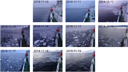
Figure 6. Sea surface temperature distribution on 9 November 2018 (left: AMSR2, right: IcePOM). White areas indicate presence of sea ice and gray areas indicate missing data.

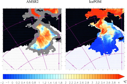
Figure 7. Vertical profiles of ocean temperature on 7 November 2018 along section A–B of cruise track indicated in Figure 1. (a) IcePOM forecast with climatological boundary conditions, (b) conductivity, temperature and depth observations from the research vessel MIRAI, and (c) IcePOM forecast with RIOPS boundary conditions.

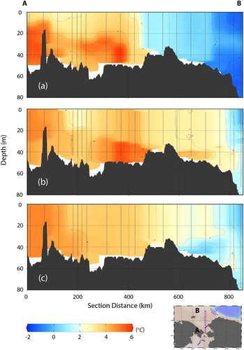
Figure 8. Same as Figure 4 but model is run with RIOPS boundary conditions.

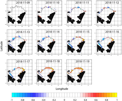
Figure 9. Evolution of ice edge errors and bias for 1–25 November 2018 from IcePOM 10-day forecast with RIOPS boundary conditions, IcePOM 10-day forecast with climatological boundary conditions, TOPAZ4 forecast, ECMWF 10-day forecast and persistence of the observations. Errors and biases were calculated with respect to Advanced Microwave Scanning Radiometer 2 (AMSR2) ((a) and (b)) and Interactive Multisensor Snow and Ice Mapping System (IMS) data ((c) and (d)). Ice edge was defined by thresholds of 15% and 40% ice concentrations for comparison with AMSR2 and IMS, respectively.

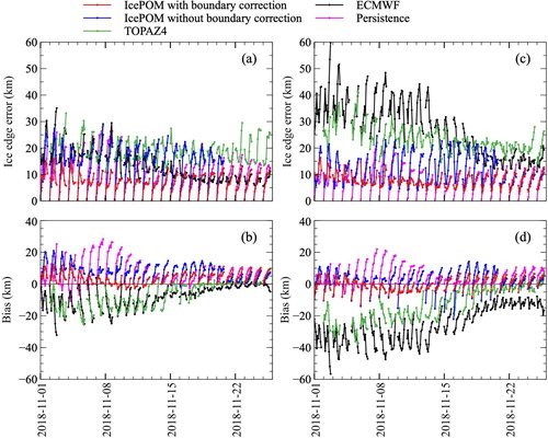
Figure 10. Evolution of IcePOM overestimation and underestimation of sea ice extent distribution for 9–19 November 2018. Forecast begins on 9 November 2018. Ice edge is indicated by a threshold ice concentration of 15%. Ice edge from Advanced Microwave Scanning Radiometer 2 (AMSR2) is shown in black contour. Color scheme is the same as that in Figure 3.

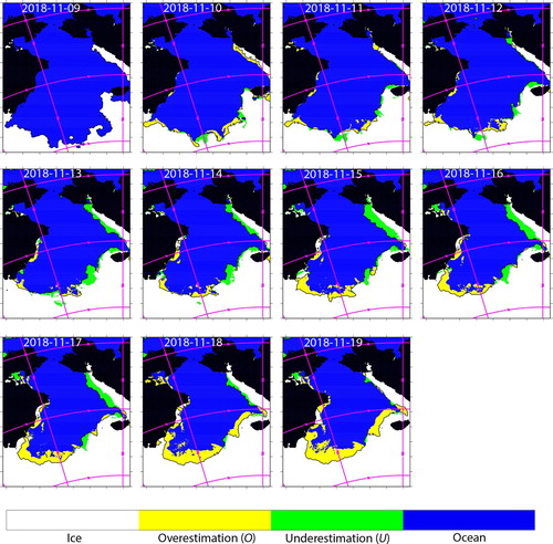
Figure 11. Time–depth cross section of ocean temperature for 10–20 November 2018 at the marginal ice zone. (a) results from conductivity, temperature and depth (CTD) observations from MIRAI, (b) RIOPS forecast, (c) IcePOM forecast with RIOPS boundary conditions, (d) IcePOM forecast with climatological boundary condition, and (e) locations of CTD observations.

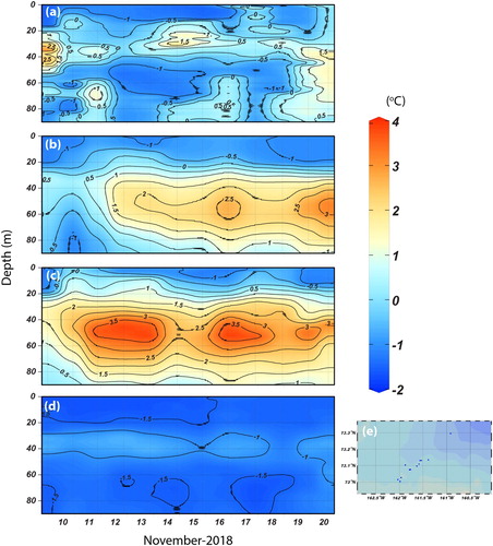
Figure 12. Time–depth cross section of ocean salinity for 10–20 November 2018 at the marginal ice zone. (a) results from conductivity, temperature and depth (CTD) observations from MIRAI, (b) RIOPS forecast, (c) IcePOM forecast with RIOPS boundary conditions, (d) IcePOM forecast with climatological boundary condition, and (e) locations of CTD observations.

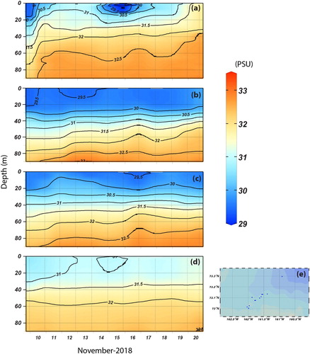
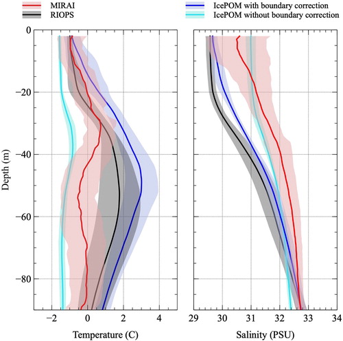
Figure 13. Time-averaged temperature and salinity profiles at the marginal ice zone for the data presented in Figures 10 and 11. Thick lines indicate average values and shading indicates standard deviation.