Prediction of daily fine particulate matter concentrations using aerosol optical depth retrievals from the Geostationary Operational Environmental Satellite (GOES)

Figures & data

Figure 1. PM_2.5 monitoring site locations within the study domain.

Table 1. Site bias (μg m^{− 3}) estimates for 26 EPA PM_2.5 monitoring sites

Site ID	City	N	Mean	CV	Bias	P value
09-001-0010	Bridgeport, CT	73	13.1	0.74	0.8	0.2
09-001-0113	Bridgeport, CT	69	12.5	0.70	0.9	0.2
09-001-1123	Danbury, CT	80	13.4	0.52	1.3	0.03
09-001-2124	Stamford, CT	74	14.2	0.66	1.2	0.04
09-001-3005	Norwalk, CT	76	13.3	0.69	1.2	0.05
09-001-9003	Westport, CT	79	12.3	0.64	0.2	0.7
09-003-1003	E. Hartford, CT	234	11.5	0.70	−0.6	0.2
09-003-1018	Hartford, CT	78	12.9	0.66	−0.1	0.8
09-009-0018	New Haven, CT	228	16.0	0.67	4.0	<0.0001
09-009-0026	New Haven, CT	69	12.1	0.70	0.4	0.5
09-009-1123	New Haven, CT	81	14.2	0.70	1.2	0.04
09-009-2008	New Haven, CT	74	12.3	0.80	−0.3	0.6
09-009-2123	Waterbury, CT	80	12.8	0.68	−0.1	0.8
09-009-8003	W. Haven, CT	74	13.0	0.79	1.5	0.01
09-011-3002	Norwich, CT	71	11.7	0.66	−1.0	0.1
25-005-1004	Fall River, MA	71	10.3	0.77	−1.0	0.2
25-009-2006	Lynn, MA	74	10.5	0.64	−2.1	0.001
25-009-5005	Haverhill, MA	68	9.4	0.65	−2.5	<0.0001
25-013-0008	Chicopee, MA	192	10.2	0.98	−2.3	<0.0001
25-013-0016	Springfield, MA	201	12.6	0.75	0.2	0.7
25-013-2009	Springfield, MA	60	11.6	0.70	−0.8	0.2
25-023-0004	Brockton, MA	82	9.7	0.71	−1.3	0.04
25-025-0027	Boston, MA	206	11.8	0.55	0.3	0.5
25-025-0042	Boston, MA	205	11.5	0.62	−1.4	0.007
25-025-0043	Boston, MA	77	13.0	0.59	0.4	0.6
25-027-0020	Worcester, MA	143	10.8	0.63	−1.1	0.004
Notes: CV represents coefficient of variation. Bias represents the random-effect estimates of the site term in the mixed-effects model.

Figure 2. The relationship between column aerosol optical depth (AOD) derived from the GOES satellite and 24-hr integrated PM_2.5 concentrations measurements at the 26 EPA sites in New England.

Figure 3. (a–c) Frequency distributions of AOD values as a function of PM_2.5 concentrations. (d–f) Frequency distribution of PM_2.5 mass as a function of AOD values.

Figure 4. Frequency distribution of the random slopes and intercepts.

Figure 5. (a, b) Mixed-effects model cross-validation performance as assessed by 576 measured and predicted daily PM_2.5 concentrations (10% of data). The solid line represents the regression line, and the dashed line displays the 1:1 line. (c) Cross-sectional comparisons between the average predicted and measured PM_2.5 site concentrations.

Table 2. Comparisons between the measured and predicted PM_2.5 concentrations using mixed-effects model

Site ID	City	N	PM2.5 Measured	PM2.5 Predicted	Bias	R ^2	Precision	% Precision
09-001-0010	Bridgeport, CT	23	13.4	12.3	−1.1	0.94	1.4	10.4
09-001-0113	Bridgeport, CT	22	11.8	10.9	−0.9	0.97	1.8	15.3
09-001-1123	Danbury, CT	25	14.3	12.5	−1.8	0.98	2.6	18.2
09-001-2124	Stamford, CT	30	15.2	13.9	−1.3	0.97	2.5	16.4
09-001-3005	Norwalk, CT	28	15.8	14.5	−1.3	0.87	2.1	13.3
09-001-9003	Westport, CT	29	13.9	13.4	−0.5	0.99	1.5	10.8
09-003-1003	E. Hartford, CT	77	12.2	12.9	0.7	0.97	2.5	20.5
09-003-1018	Hartford, CT	24	12.2	12.3	0.1	0.97	1.2	9.8
09-009-0018	New Haven, CT	72	17.4	13.8	−3.6	0.96	6.9	39.7
09-009-0026	New Haven, CT	27	14.4	14.0	0.4	0.99	1.3	9.0
09-009-1123	New Haven, CT	31	15.4	14.0	−1.4	0.98	2.1	13.6
09-009-2008	New Haven, CT	29	14.0	14.3	0.3	0.99	1.7	12.1
09-009-2123	Waterbury, CT	28	13.9	13.9	0	0.99	1.4	10.1
09-009-8003	W. Haven, CT	28	16.8	15.1	−1.7	0.98	3.9	23.2
09-011-3002	Norwich, CT	24	13.8	14.6	0.8	0.98	1.3	9.4
25-005-1004	Fall River, MA	20	10.7	11.0	0.3	0.96	3.2	29.9
25-009-2006	Lynn, MA	22	10.6	11.8	1.2	0.80	4.3	40.6
25-009-5005	Haverhill, MA	21	10.4	12.2	1.7	0.95	2.9	27.9
25-013-0008	Chicopee, MA	63	9.1	11.6	2.5	0.96	3.6	39.6
25-013-0016	Springfield, MA	65	12.8	12.6	−0.2	0.93	2.5	19.5
25-013-2009	Springfield, MA	20	10.6	11.5	1.3	0.98	1.6	15.1
25-023-0004	Brockton, MA	22	9.6	11.0	1.4	0.99	3.4	35.4
25-025-0027	Boston, MA	69	12.7	12.4	−0.3	0.76	4.1	32.2
25-025-0042	Boston, MA	61	11.7	13.1	1.4	0.98	3.1	26.5
25-025-0043	Boston, MA	19	14.9	14.2	−0.7	0.97	2.0	13.4
25-027-0020	Worcester, MA	47	11.0	13.1	2.1	0.97	3.2	29.1
Notes: N indicates the number of days with both measured and predicted PM2.5 concentrations. Bias is defined as (PM2.5 predicted − PM2.5 measured). Precision is estimated as the square root of the mean of the squared errors. % Precision is defined as [100 × (precision/PM2.5 measured)].

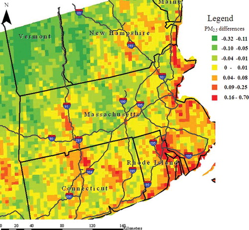
Figure 6. Spatial variability in PM_2.5 levels in the study region. Note that PM_2.5 levels are expressed as differences between grid-specific predicted and regional PM_2.5 concentrations (µg m⁻³).