Evaluating the effects of climate change on summertime ozone using a relative response factor approach for policymakers

Figures & data

Figure 1. Semi-hemispheric and continental U.S. (CONUS) CMAQ modeling domains.

Figure 2. Definition of the regions used in summarizing results.

Figure 3. Percent change in continental U.S. emissions from the present-day to the 2050s by region. BVOC represents biogenic VOC emissions that are allowed to change with the future climate.

Table 1. Matrix of 36-km CONUS domain CMAQ simulations

Simulation name	Meteorology	Anthropogenic emissions	Biogenic emissions
CD_Base	Current	NEI 2002	Current meteorology
FD_US	Current	MARKAL 2050	Current meteorology
A1B_Met	Future	NEI 2002	Current meteorology
A1B_M	Future	NEI 2002	Future meteorology
A1B_US_Met	Future	MARKAL 2050	Current meteorology
A1B_US_M	Future	MARKAL 2050	Future meteorology
Note: Future meteorology is based on the IPCC A1B scenario. NEI 2002 refers to the U.S. EPA National Emissions Inventory for 2002. MARKAL 2050 refers to a future emissions inventory that is based on the NEI 2002 and projected to 2050 using the U.S. EPA MARKAL allocation model. The same present-day chemical boundary conditions from the semi-hemispheric CMAQ simulations are used for all cases. All simulations use present-day land-use and land-cover data. Chemical boundary conditions are held constant at present-day levels for all simulations.

Figure 4. Simulated change in meteorological parameters due to climate change. Percent change in temperature (˚C) and PBL are from average daily maximum values, while water vapor, precipitation, insolation, and wind speed are from average values.

Figure 5. Observed (open dark circles) and modeled (open gray circles) daily maximum hourly ozone as a function of summertime daily maximum hourly temperature at 72 CASTNET sites. The data have been grouped by site location based on the region definitions in Figure 2. The observed and modeled linear best-fit lines are shown as solid and dashed, respectively. The slope of the linear best-fit is shown in the upper-left corner of each tile [ppb/˚C].

Figure 6. Simulated change in average daily maximum temperature and the corresponding change in average daily maximum 1-hr ozone at the 72 CASTNET sites when biogenic emissions are held constant (A1B_Met; solid circles) and when biogenic emissions are allowed to change in response to the future climate (A1B_M; open squares).

Table 2. Summary of RRF_E by region

		RRFE
Region	Number of sites	Average	Minimum	Maximum	Standard deviation	Percent of sites with RRF >1.00
Northwest	11	0.95	0.92	0.97	0.021	0
Southwest	246	0.91	0.85	1.07	0.043	5
Central	31	0.92	0.86	0.98	0.030	0
South	124	0.95	0.88	1.02	0.040	9
Midwest	287	0.95	0.91	1.00	0.019	0
Southeast	211	0.91	0.84	0.99	0.027	0
Northeast	225	0.92	0.85	1.16	0.048	3
All regions	1135	0.93	0.84	1.16	0.040	3

Figure 7. Spatial map of the RRF_E for the 1135 ozone monitoring locations in which the CD_Base case had at least one day where the daily maximum 8-hr ozone exceeded 75 ppb. Values less than one imply a reduction in daily maximum 8-hr ozone, while values greater than one imply an increase in daily maximum 8-hr ozone when anthropogenic emissions are reduced as shown in Figure 3 (color figure available online).

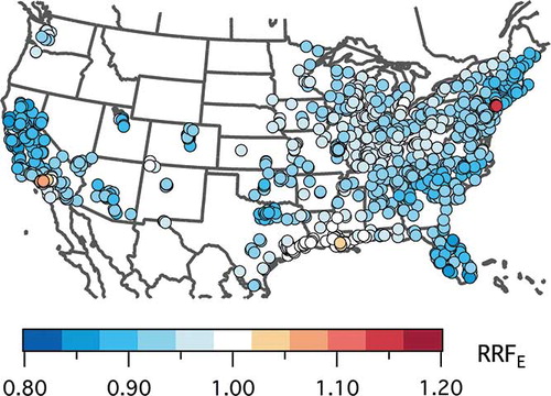
Table 3. Summary of climate-adjusted RRFs ( eqs (4) and (5)) by region

		RRFEC (RRFECB)
Region	Number of sites	Average	Minimum	Maximum	Standard deviation	Percent of sites with RRF >1.00
Northwest	11	0.87	0.84	0.89	0.020	0
		(0.87)	(0.84)	(0.89)	(0.017)	(0)
Southwest	246	0.91	0.82	1.09	0.059	7
		(0.92)	(0.83)	(1.15)	(0.070)	(13)
Central	31	0.97	0.88	1.07	0.066	42
		(0.98)	(0.87)	(1.10)	(0.074)	(42)
South	124	1.04	0.94	1.16	0.057	66
		(1.05)	(0.94)	(1.22)	(0.071)	(65)
Midwest	287	1.04	0.97	1.13	0.033	89
		(1.05)	(0.94)	(1.18)	(0.047)	(88)
Southeast	211	0.99	0.85	1.07	0.039	31
		(0.97)	(0.85)	(1.11)	(0.040)	(22)
Northeast	225	1.00	0.91	1.25	0.057	32
		(1.00)	(0.90)	(1.34)	(0.074)	(30)
All regions	1135	0.99	0.82	1.25	0.069	45
		(1.00)	(0.83)	(1.34)	(0.079)	(43)

Figure 8. Climate adjustment factor (CAF_CB) for the A1B_US_M case (top), and the associated climate adjusted RRF (RRF_ECB; bottom). A CAF is calculated for all sites, but not all sites have an RRF (color figure available online).

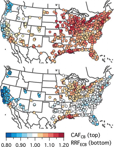
Figure 9. Simulated average daytime NO_X as a function of average daytime VOC at ozone monitoring sites for the A1B_US_Met case. Data points are color coded based on the ratio of the average daily maximum 8-hr O₃ from the A1B_US_M and A1B_US_Met cases. The size of each data point represents the ratio of average daytime organic nitrates (RNO₃) concentration in the A1B_US_M and A1B_US_Met cases (color figure available online).

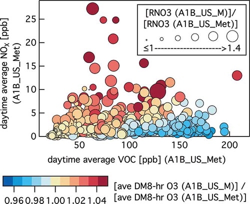
Figure 10. (a) Comparison between CAF_C and CAF_CB ( eqs (2) and (3)), when future anthropogenic emissions are used (A1B_US_M and A1B_US_Met cases), and when current anthropogenic emissions are used (A1B_M and A1B_Met cases). (b) Comparison between RRF_E from eq (1) when the RRF is calculated under the current climate (CD_Base and FD_US cases) and under the future climate (A1B_Met or A1B_M and A1B_US_Met and A1B_US_M cases, respectively).

Figure 11. Comparison of the climate adjustment factor (CAF_CB) from this study with that calculated from the work of Avise et al. (2008) and Chen et al. (2009), when current anthropogenic emissions are used and biogenic emissions are allowed to change with the future climate (i.e., alternate CAF methodology is used).

Avise , J. , Chen , J. , Lamb , B. , Wiedinmyer , C. , Guenther , A. , Salathé , E. and Mass , C. 2008 . Attribution of projected changes in summertime U.S. ozone and PM2.5 concentrations to global changes . Atmos. Chem. Phys. , 8 : 15131 – 15163 .

 Google Scholar

Chen , J. , Avise , J. , Guenther , A. , Wiedinmyer , C. , Salathé , E. , Jackson , R.B. and Lamb , B. 2009 . Future Land Use and Land Cover Influences on Regional Biogenic Emissions and Air Quality in the United States . Atmos. Environ. , 43 : 5771 – 5780 . doi: 10.1016/j.atmosenv.2009.08.015

 Web of Science ®Google Scholar