612
Views
5
CrossRef citations to date
0
Altmetric
Notebook Paper

Evaluating the performance of the horizontal radial plume mapping technique for locating multiple plumes

&
Pages 1249-1256 | Published online: 24 Oct 2012

Figures & data

Figure 1.(a) The plan view of the simulated beam geometry. The letters A to I represent the pixel IDs, and the numbers in parenthesis represent the beam IDs. (b) An example of the test map with two Gaussian distributions (SD = 2). (c) The reconstruction results of (b) by the NNLS algorithm. (d) An example of the test map with two Gaussian distributions (SD = 4). (e) The reconstruction results of (d) by the NNLS algorithm. The grayscale bars represent the relative concentration levels of the reconstructed plumes.
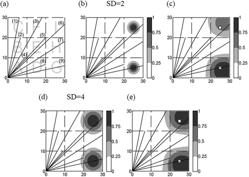
Figure 1.(a) The plan view of the simulated beam geometry. The letters A to I represent the pixel IDs, and the numbers in parenthesis represent the beam IDs. (b) An example of the test map with two Gaussian distributions (SD = 2). (c) The reconstruction results of (b) by the NNLS algorithm. (d) An example of the test map with two Gaussian distributions (SD = 4). (e) The reconstruction results of (d) by the NNLS algorithm. The grayscale bars represent the relative concentration levels of the reconstructed plumes.

Table 1. Summary statistics of the NNLS reconstruction results for test maps with SD = 2

Figure 2.Examples of the reconstruction results for the test maps with two plumes in close proximity to each other. First column (a, d, g, j): Test maps. Second column (b, e, h, k): The NNLS reconstruction results. Third column (c, i): The SBFM reconstruction results; (f, l): the NNLS-GT reconstruction results. The white squares represent the real-source locations. The grayscale bars represent the relative concentration levels of the reconstructed plumes.
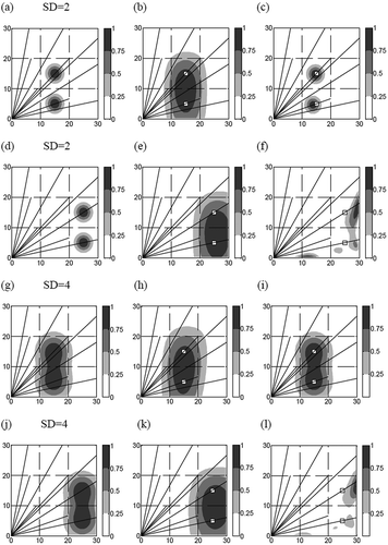
Figure 2.Examples of the reconstruction results for the test maps with two plumes in close proximity to each other. First column (a, d, g, j): Test maps. Second column (b, e, h, k): The NNLS reconstruction results. Third column (c, i): The SBFM reconstruction results; (f, l): the NNLS-GT reconstruction results. The white squares represent the real-source locations. The grayscale bars represent the relative concentration levels of the reconstructed plumes.

Figure 3.Examples of the reconstruction results from the NNLS and SBFM algorithms for test maps with one of the simulated plumes close to the origin. First column: Test map. Second column: The corresponding NNLS reconstruction results. Third column: The corresponding SBFM reconstruction results. The white square represents the real-source location. The grayscale bars represent the relative concentration levels of the reconstructed plumes.
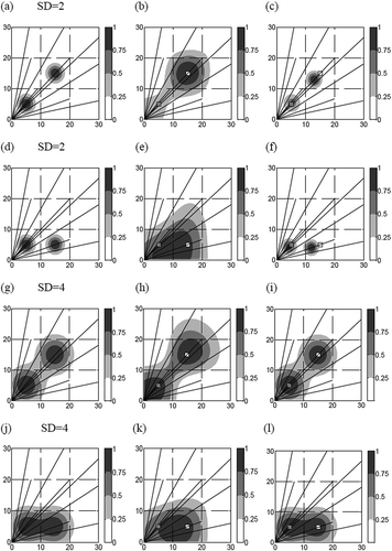
Figure 3.Examples of the reconstruction results from the NNLS and SBFM algorithms for test maps with one of the simulated plumes close to the origin. First column: Test map. Second column: The corresponding NNLS reconstruction results. Third column: The corresponding SBFM reconstruction results. The white square represents the real-source location. The grayscale bars represent the relative concentration levels of the reconstructed plumes.

Figure 4.Examples of the reconstruction results for test maps with three plumes. (a, b, c) The plumes are away from the origin. (d, e, f) The plumes are close to the origin. The white squares represent the real-source locations. The grayscale bars represent the relative concentration levels of the reconstructed plumes.
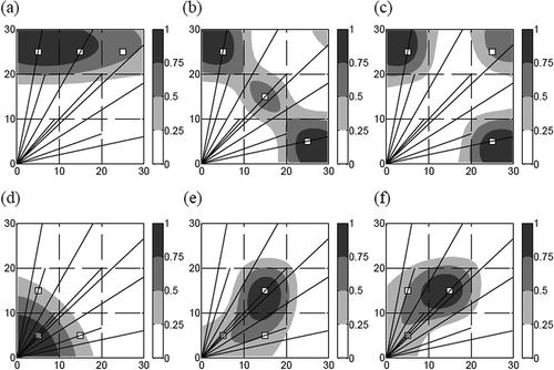
Figure 4.Examples of the reconstruction results for test maps with three plumes. (a, b, c) The plumes are away from the origin. (d, e, f) The plumes are close to the origin. The white squares represent the real-source locations. The grayscale bars represent the relative concentration levels of the reconstructed plumes.
Supplemental material

uawm_a_710552_sup_27792985.pdf

Download PDF (23.7 KB)

Reprints and Corporate Permissions

Please note: Selecting permissions does not provide access to the full text of the article, please see our help page How do I view content?

To request a reprint or corporate permissions for this article, please click on the relevant link below:

Academic Permissions

Please note: Selecting permissions does not provide access to the full text of the article, please see our help page How do I view content?

Obtain permissions instantly via Rightslink by clicking on the button below:

If you are unable to obtain permissions via Rightslink, please complete and submit this Permissions form. For more information, please visit our Permissions help page.