Figures & data
Table 1. Meteorological specifications for the fifth-Generation Pennsylvania State University–National Center for Atmospheric Research Mesoscale Model (MM5) and the Weather Research and Forecasting (WRF) model
Figure 1. Radar wind profiler locations (blue squares) and major cities (red circles) in eastern Texas during the TexAQS II field campaign. Color shading shows terrain elevation (CitationWilczak et al., 2009). (Color figure available online).
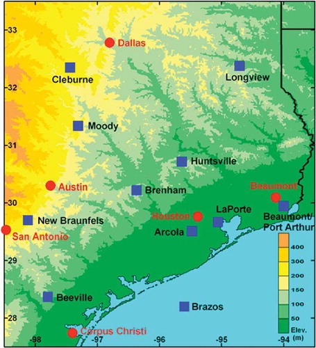
Figure 2. Location of the UH Moody Tower measurement site in downtown Houston (Reprinted with permission from Google, Copyright 2012).
Figure 3. Root mean square error for each RWP station location (ordered furthest inland on the left to nearest to the coast on the right) for the (a) morning rise PBL height (8 a.m.–11 a.m.), (b) afternoon peak PBL height, and (c) evening collapse PBL height (4 p.m.–7 p.m.).
Table 2. Ten radar wind profiler stations divided into three categories based on geographic location
Figure 4. Time series of the median hourly PBL height (m) over the entire episode for RWP locations in (a) central Texas, (b) inland, and (c) the coastal plains.
Figure 5. Time series of median 2-m temperature (left) and 2-m water vapor mixing ratio (right) over the entire episode period for (a) central Texas, (b) inland, and (c) coastal plains.
Figure 6. Time series of median sensible heat flux (left) and latent heat flux (right) over the entire episode period for (a) central Texas, (b) inland, and (c) coastal plains.
Figure 7. Time series of modeled and observed PBL heights on September 7, 2006, at Moody Tower, Houston. Open circles indicate visually estimated PBL heights from the lidar backscatter image, and green diamonds indicate visually estimated PBL heights from radiosonde profiles.
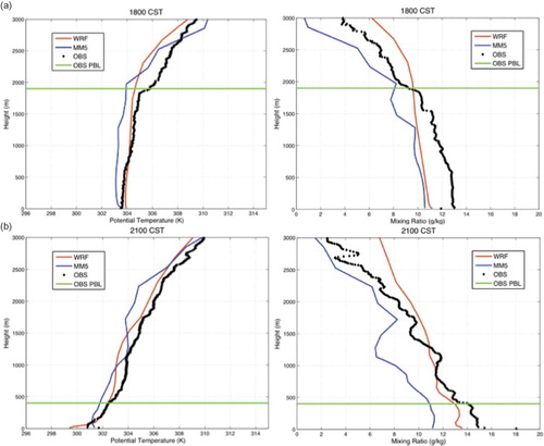
Figure 8. Vertical profiles of potential temperature (left) and mixing ratio (right) as recorded from radiosonde balloons launched at Moody Tower, Houston, on September 7, 2006, at (a) 09:00 a.m., (b) 12:00 p.m., and (c) 3:00 p.m. CST. (Color figure available online).
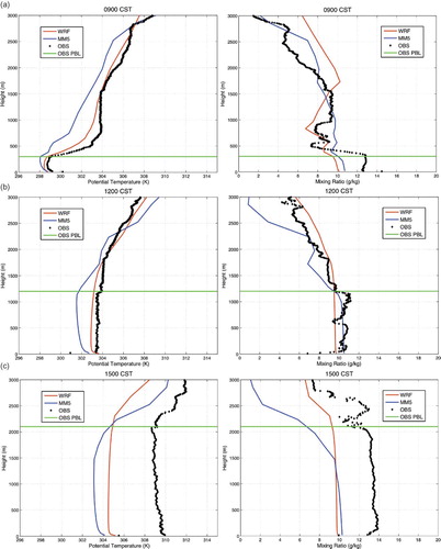
Figure 9. Vertical profiles of potential temperature (left) and mixing ratio (right) as recorded from radiosonde balloons launched at Moody Tower, Houston, on September 7, 2006, at (a) 3:00 p.m., (b) 6:00 p.m., and (c) 9:00 p.m. CST. (Color figure available online).