An uncertainty analysis of mean flow velocity measurements used to quantify emissions from stationary sources

Figures & data

Figure 1. (a) Natural-gas burner under the largest of three exhaust hoods (1, large, 9 m × 12 m; 2, medium, 6 m × 6 m; 3, small, 3 m × 3 m). (b) Portion of the exhaust duct on the roof of the facility and upstream of the pollution control system.

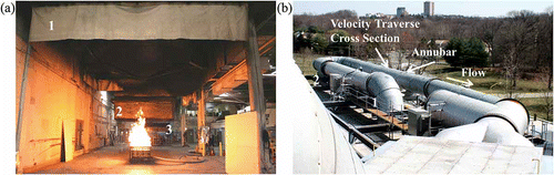
Figure 2. View of the velocity traverse plane located 9.2 D downstream of 180º bend, and the Annubar located 2.9 D downstream of traverse plane.

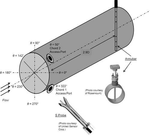
Figure 3. CFD mesh showing the geometry of the exhaust duct and the location of the traversing plane relative to the 180° bend in the duct.

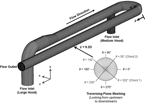
Table 1. Uncertainty budget for Series 1 point velocity measurements

Measurement component, xi	Value	Relative standard uncertainty, u(xi)/xi	Nondimensional sensitivity coefficient, si	Percent contribution, %
Probe coefficient, Cp	0.818	0.0048	1.0	86.7
Probe yaw, (deg)	2.49	0.0201	0.002	0
Probe differential pressure, Δp (Pa)	110.38	0.0008	0.5	0.5
Gas temperature, T (K)	296	0.0037	0.5	12.8
Duct static pressure, Ps (Pa)	100722	0.0001	−0.5	0
Gas molecular weight, Mwet (kg/kmol)	28.297	0.0001	−0.5	0
Near axial velocity, vz (m/sec)	11.28	0.0052 (0.0104)	Standard uncertainty (Expanded uncertainty)

Figure 4. Measured (symbols) and simulated (dashed line) velocity distributions on chord 1 and chord 2 for ambient (open symbols) and heated (closed symbols) flow conditions, with flow starting at the large hood. The natural gas burner is located under the southwest (SW) corner of the exhaust hood. The uncertainty bars correspond to a 95% confidence interval; the nominal value is listed in Table 1.

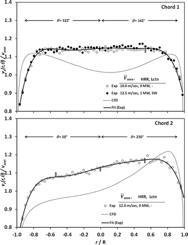
Table 2. Uncertainty budget for Series 2 point velocity measurements, with standard uncertainty estimates derived from EPA (Method 2 or 2G) and ASTM (D 3154) standard test methods

Measurement component, xi	Value	Standard uncertainty, u(xi)	Relative standard uncertainty, u(xi)/xi	Nondimensional sensitivity coefficient, si	Percent contribution, %
Probe coefficient, Cp	0.785	0.012	0.0150 ^b^, ^c	1.0	88.5
Probe yaw, (deg)	2.0	0.5 ^b	0.2500	0.002	0
Probe differential pressure, Δp (Pa)	403.6	3.1 ^b	0.0077	0.5	5.8
Gas temperature, T (K)	287.3	1.5 ^b	0.0052	0.5	2.7
Duct static pressure, Ps (Pa)	99193	170 ^a,b	0.0017	−0.5	0.3
Gas molecular weight, Mwet (kg/kmol)	28.73	0.15 ^c	0.0052	−0.5	2.7
Near axial velocity, vz (m/sec)	20.41	0.33 (0.65)	0.0159 (0.0319)	Standard uncertainty (Expanded uncertainty)

Notes: ^aEPA Method 2.

^bEPA Method 2G.

^cASTM D3154.

Figure 5. Series 2 velocity profiles for ambient flow conditions in the large exhaust hood. Sample locations correspond to centroid of equal area positions. The uncertainty bars correspond to a 95% confidence interval; the range of uncertainty is stated in the associated text.

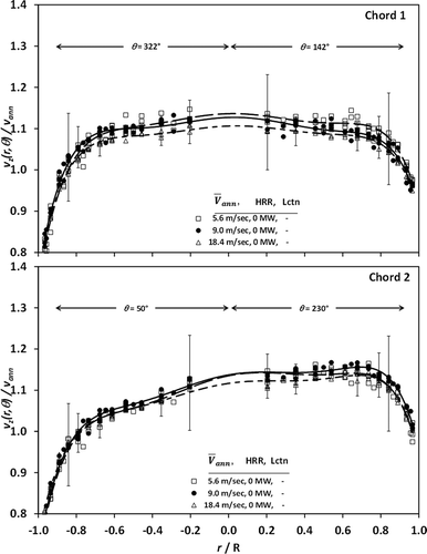
Figure 6. Series 2 velocity profiles for heated flow conditions in the large exhaust hood. Sample locations correspond to centroid of equal area positions. The natural gas burner was located under the southwest (SW) corner as well as the center (C) of the exhaust hood. The uncertainty bars correspond to a 95% confidence interval; the range of uncertainty is stated in the associated text.

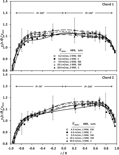
Figure 7. Slice view of axial velocity at z = 9.2D downstream of the 180° bend.

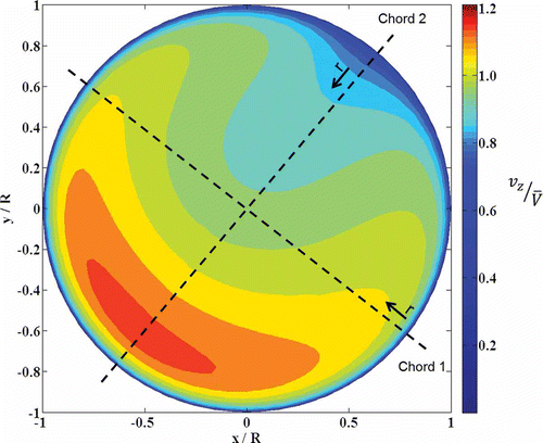
Figure 8. Distribution of discretization error with orientation of traverse chords.

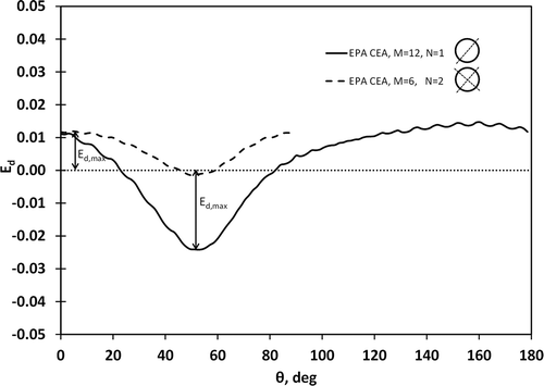
Figure 9. Range of maximum potential discretization error with respect to number of sampling locations, number of sampling chords, and numerical integration technique.

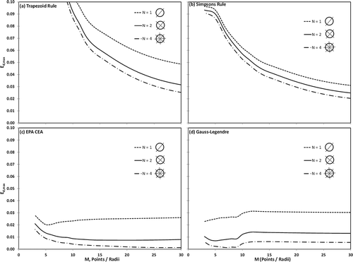
Figure 10. Comparison of mean flow velocity computed as an arithmetic average (EPA) and as the result of numerical integrations (trapezoid, Simpsons, and Gauss–Legendre). The uncertainty bars correspond to a 95% confidence interval; nominal values are listed in Table 3.

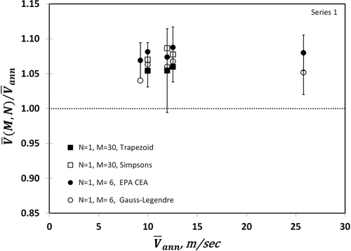
Table 3. Nominal values for the relative uncertainty, , of the estimate for mean flow velocity

	Series 1					Series 2
	N	M				N	M
EPA CEA	1	6	0.002	0.013	0.013 (0.026)	2	12	0.005	0.005	0.007 (0.014)
Gauss	1	6	0.002	0.016	0.016 (0.032)	2	12	0.005	0.008	0.009 (0.019)
Simpsons	1	30	0.003	0.020	0.020 (0.040)	2	12	0.006	0.030	0.031 (0.062)
Trapezoid	1	30	0.003	0.030	0.030 (0.060)	2	12	0.006	0.046	0.046 (0.093)

Note: Values in parentheses are relative expanded uncertainty.

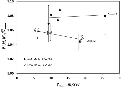
Figure 11. Comparison of Series 1 and Series 2 mean flow velocity measurements. The uncertainty bars correspond to a 95% confidence interval; nominal values are listed in Table 3.