Emission factors for fugitive dust from bulldozers working on a coal pile

Figures & data

Figure 1. Environs surrounding the coal pile (oval black area) at the Tennessee study site. The photograph is oriented north-south from top to bottom. Monitoring sites are denoted by green circles.

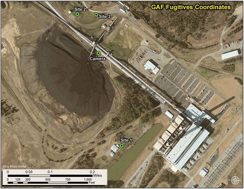
Table 1. Average adjusted PM₁₀ concentration C_xs* for hours without and with human activity on the coal pile

Monitoring site	Concentration, µg m^−3
	Without activity	With activity
2	19.7	60.7
3	21.1	59.9

Table 2. Comparison of fugitive PM₁₀ concentrations^a associated with natural and human activity on a coal pile (data from both downwind sites combined)

Variable	PM10 concentration statistic, µg m^−3
	Maximum	Mean	Median	Geometric mean
Cxs*	1196	60.3	33.1	33.8
	130	40.8	36.5	34.2
	1066	31.2	2.6	5.3

Note: ^aConcentrations were adjusted to reflect levels associated with continuous airflow over the source.

Figure 2. Frequency distributions of C_xs* (top), (middle), and (bottom) for hours when airflow transported bulldozer-derived dust from the coal pile toward downwind monitors. Bin labels indicate the midpoint of each 20-µg m⁻³ range in bin values.

Figure 3. Coal pile direction sectors (numbered 1 through 3) and subsectors (labeled “a” and “b” within each direction sector) for which hourly bulldozer activity was quantified by use of camera imagery. The camera was initially oriented to acquire images within the yellow-delineated field of view but was adjusted (red delineation) to capture a more central field of view—and more of sector 3—in September.

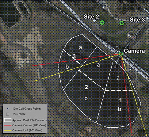
Table 3. Average observed frequencies (weights) used to allocate simulated fugitive dust emissions to each coal pile sector

Frequency	Downwind site	Coal pile sector
		1a	1b	2a	2b	3a	3b
Airflow across pile^a	2	0.35		0.27		0.19
	3	0.41		0.18		0.15
Pile activity^b	—	0.41	0.31	0.10	0.14	0.02	0.01
Airflow × activity^c	2	0.42	0.28	0.10	0.14	0.05	0.01
	3	0.45	0.29	0.10	0.11	0.03	0.01

Notes: ^aAverage frequency during each hour that the observed 1-min 10-m wind aligned a 30° coal-pile direction sector with a downwind site. Values in this row do not sum to 1.00 because of the minutes when airflow did not cross the pile (off-pile frequencies were 0.19 for site 2 and 0.26 for site 3).

^bObserved frequency of total hourly bulldozer activity that occurred within a coal pile sector. Row does not sum to 1.00 due to rounding.

^cJoint frequency of airflow and pile activity occurring relative to a downwind monitor. Rows may not sum to 1.00 due to rounding.

Table 4. Sector-specific meteorological conditions at 10 m averaged for periods when airflow over the coal pile aligned with downwind monitoring sites

Site: sector	θ10 (deg.)	σθ (deg.)	u10 (m s^−1)	σw (m s^−1)	TKE^a (m^2 s^−2)
2: 1	168	15.4	1.66	0.28	0.19
2: 2	195	17.2	1.80	0.33	0.23
2: 3	228	17.3	1.74	0.31	0.20
3: 1	179	15.6	1.77	0.30	0.20
3: 2	208	18.5	1.71	0.34	0.23
3: 3	238	16.8	1.71	0.30	0.19

Note: ^aPer unit mass.

Table 5. Source characteristics used to model area emissions from the coal pile

Characteristic	Pile sector
	1a	1b	2a	2b	3a	3b
Area (ha)	0.72	1.15	1.09	1.09	0.69	0.46
Mean source elevation^a (m)	0	0	0	0	0	15
Initial plume depth^b (m)	2	15	2	15	12	2
Distance (m) from sector center to site 2	225	306	170	265	146	207
Distance (m) from sector center to site 3	214	299	187	285	214	255

Notes: ^aHeight relative to pile base.

^bThe minimum depth was roughly the height of the bulldozer. Larger values were selected to model dispersion from sectors in which the variation in pile elevation caused bulldozers to drive from lower to higher points on the pile.

Figure 4. Distribution of observed bulldozer activity (total minutes) per hour. Bin labels are the upper end of the 10-min range in bin values with up to two bulldozers working at once.

Table 6. Calculated nonzero PM₁₀ coal dust emission rates due to bulldozer activity

Metric	Site 2	Site 3
Sample size	139	150
Mean Qf10, g ha^−1 sec^−1	5.5	3.2
Median Qf10, g ha^−1 sec^−1	0.09	0.10
Median Qe, kg hr^−1	0.76	0.71
Median Ev, kg min^−1	0.016	0.022
Geometric mean Ev, kg min^−1	0.026^a
AP-42 Ev from mean S, kg min^−1	0.121^a
Geometric mean of AP-42 Ev, kg min^−1	0.131^a

Note: ^aData from both downwind sites combined.

Figure 5. Plot compares daily average log₁₀(E_v) versus M_c for separate periods either ending before or beginning on October 15. Separate linear regression lines (and coefficients of determination) are shown for each period. The two lines intersect at roughly M_c = 29.5%.

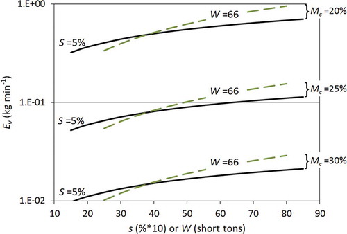
Figure 6. Comparison of different values of E_v versus M_c using emission factors from AP-42 for unpaved public roads, unpaved industrial surfaces, and from this study. The potential variability of the E_v(AP) for industrial sites—assuming 25% variability in vehicle speed and surface silt content—is illustrated using dashed lines above and below the parallel solid line.

Figure 7. Daily average coal moisture content for 2012 computed from hourly meteorological data measured near Nashville, TN, and eq 22. The period of the field study is denoted by the solid horizontal line in the upper part of the graph.

Figure 8. Daily emission factors for fugitive PM₁₀ coal dust calculated using the formulations for E_v versus M_c (eqs 23 and 24) and M_c plotted in Figure 7. The period of the field study is denoted by the solid horizontal line in the upper part of the graph. The E_v(AP) (= VE_ir) is represented by the horizontal dashed line near 100 g min⁻¹, and the annual average of E_v based on the study formulation is represented by the dashed line parallel to and below the line for E_v(AP).

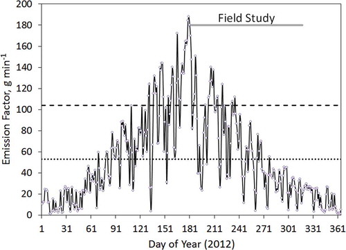
Figure 9. Sensitivity of E_v to various independent variables as determined from eq 27.