A comparison of correlation-length estimation methods for the objective analysis of surface pollutants at Environment and Climate Change Canada

Figures & data

Table 1. Terminology of data assimilation.

Terminology	Explanation
Analysis	Best representation of air quality over an area, resulting from combining all available observations with an air quality model (called the prior). The analysis is sometime called the posterior.
Objective analysis	The term “objective” has an historical origin; it is simply a reminder that the analysis is produced objectively using an estimation method or algorithm rather than by hand by a meteorologist or an air quality expert, which would then be called a subjective analysis.
Data assimilation	A cycle of analyses and forecasts that runs over time. Data assimilation effectively accumulates observation information from the past up to the current time, and thus provides a more accurate depiction of the state of the atmosphere. It is different from a single analysis that provides basically a snapshot at a given time.
Data fusion	The combination of observations and information from different sources and proxies, such as land use, population density, proximity of major roads, etc., to produce a better depiction of the atmospheric state. This is done typically by using statistical methods and graphical information systems (GIS). However, it does not use a predictive air quality model, nor does it use the “analysis” to initialize an air quality model, and thus should not be confused with data assimilation.
Correlation length	The distance by which the correlation function reaches a given a prescribed value (here set at 0.606). The correlation function represents the influence function in space of a correction due to a single point observation. The prescribed value is somewhat arbitrary, but in data assimilation it is becoming common to use the correlation value of a Gaussian correlation function for a (dimensionless) length-scale parameter value equal to 1.
Correlation length-scale parameter	The value of a length-scale parameter that appears in a particular correlation function. It is not equal to the decorrelation length that the particular correlation function will display. Sometimes the terminology correlation length and correlation length-scale parameter are used interchangeably, but this creates confusion.
Spatially homogeneous correlation	A spatial correlation pattern (usually horizontal) that does not change when evaluated with respect to a different reference point. Mathematically, it means that the correlation is invariant under translation of the coordinates, that is, .
Spatially isotropic correlation	A spatial correlation pattern (usually horizontal) that is identical in any direction from a reference point. Mathematically, it means a correlation that is invariant under any rotation of the coordinate system.
Gaussian correlation model	Basically a spatial correlation model whose dependence on distance r has the form . It is also known as the squared-exponential model, and should not be confused with a Gaussian probability function
Innovations	This is a term that comes from that Kalman filter theory and means the portion of the observation signal that is not already explained by the prior. In data assimilation we refer it to the observed-minus-model (or forecast) residuals.
Observation space	The ensemble of location of the observations and the physical quantities being measured that are used to form an analysis. In contrast with the model space that is generally a gridded space of the model grid points, the observation space is nonuniform and heterogeneous, and has its own characteristics for each observation types (e.g., Airnow surface observation network, satellite derived AOD, etc.).
Background	Means the state of a prognostic air quality model at a given time. In data assimilation it is the prior over which observations are combined to yield an analysis.
Kalman filter	A data assimilation method that propagates and updates its state estimate and associated error covariance over time and as it processes observations. The observations will in general reduce the uncertainties while the model may increase it over time due to a model error growth. In data assimilation the Kalman filter is prohibitive, and alternative formulations such as ensemble based formulation have been developed. For chemical data, assimilation sequential filters are another computationally efficient alternative.
Sequential filter	A simplified Kalman filter where only error variances are evolved by transport and updated by observations. It is a scheme used principally in chemical data assimilation.
3D Var, 4D Var	Methods to produce an analysis using a variational approach, and that are performed numerically by minimizing some cost function. 3D Var means that the analysis is obtained in the three-dimensional physical space. 4D Var uses the prognostic model to produce a spatial and temporal analysis, given all observations available in a time window.

Figure 1. Typical operational product of the objective analysis for O₃, June 15, 2014, 12 UTC. Upper left panel displays the model prior from GEM-MACH. The upper right panel is the analysis valid at the same time. The lower left panel is analysis increment, that is, the difference between the analysis and the model prior, and the lower right panel is the observations used to produce this analysis.

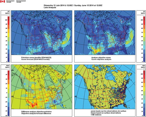
Figure 2. Correlation functions as a function of the (dimensionless) distance for common correlations models. The lower panel displays the distance dependence when the length-scale parameter of the individual models is set to unity. The upper panel shows the correlation functions when the length-scale parameter has been scaled to provide the same (unit) correlation length based on the Gaussian correlation model. Note that the solid black line (Gaussian) is identical in both panels. The vertical dashed line represents the distance at which the compact support correlation of Gaspari and Cohn is equal to zero.

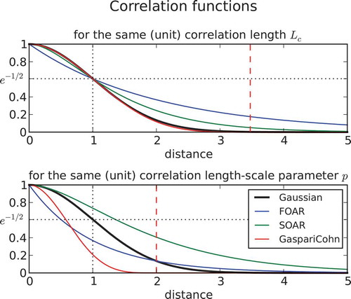
Figure 3. Example of a local Hollingsworth–Lönnberg fit of a Gaspari and Cohn correlation function for O₃ around the station Toronto North (corner of Yonge and Finch avenues) for July 2014, 16 UTC. The lower panel shows the surrounding stations where innovations are collected, with concentric circles of 100 km apart (in light green). The upper panel shows the normalized autocovariance function as function of radial distance. The fitted correlation function is displayed with a solid black line.

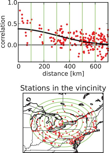
Figure 4. One-dimensional nonhomogeneous model. Left, coordinate transformation . Right, resulting nonhomogeneous correlation (with , p = 0.11, L_c = 500 km in the displaced coordinate equation, eq 7). Contour isolines (0.2, 0.4, 0.6, 0.8, 1.0).

Figure 5. HL local estimates for and . The true background error has an homogneous isotropic correlation and spatially varying variance (wavenumber 5). Squares are the true values, and filled circles are the HL estimates.

Figure 6. HL local estimates for and . The true background error has a homogeneous isotropic correlation with a spatially uncorrelated (random) background error variance. Squares are the true values, and filled circles are the HL estimates.

Figure 7. Same as Figure 5 but for a nonhomogeneous error correlation for the truth.

Figure 8. Same as Figure 6 but for a nonhomogeneous error correlation for the truth.

Figure 9. Different correlation length estimates. Spatially random error variance with nonhomogeneous error correlation as in Figure 8. Dotted-pink line represents the log-likelihood function, and in solid pink the minimum of the log-likelihood function. The mean HL local correlation length is in blue. The for different modeled correlation lengths (in abcissa) is represented with a solid black line. The ordinate are values of .

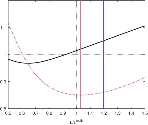
Figure 10. Distribution of the local Hollingsworth–Lönnberg correlation length estimates for O₃, NO₂, and PM_2.5 using the filtered data at 16 UTC. The blue lines represent the median and the red line the mean value.

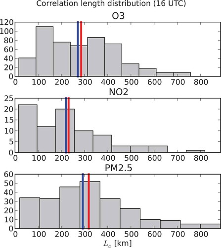
Table 2. Correlation length estimates (km) from different methods, July 2014, 16 UTC.

Species	Maximum likelihood	HL harmonic mean		HL global	Median HL
O3	155	195	227	277	265
PM2.5	215	191	295	297	303
NO2	69	107	99	225	208

Figure 11. Comparison of different correlation length estimates for O₃, NO₂, and PM_2.5 at 16 UTC for the summer 2014. in solid black, the log-likelihood function (rescaled) in dotted pink, the maximum likelihood estimate in solid pink, the global HL estimate in green, the median HL in blue, and the harmonic mean HL is in cyan.

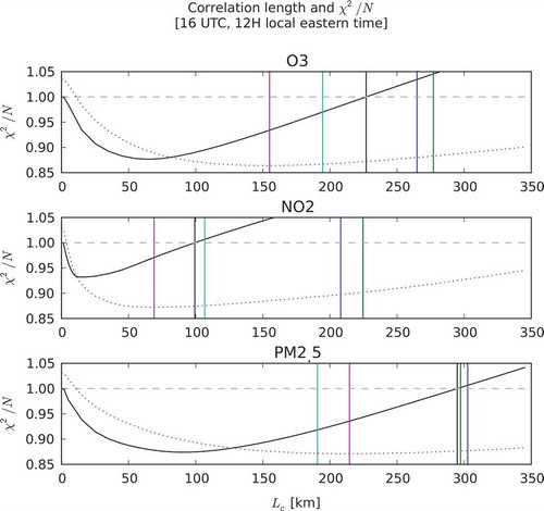
Figure 12. Time evolution of the correlation length for O₃. Maximum likelihood estimates in pink, estimates in black, and global HL in green.

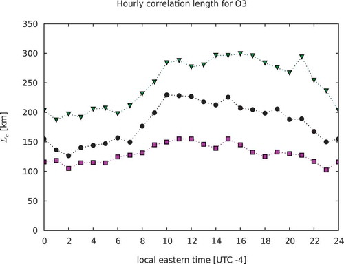
Figure 13. Time evolution of the correlation length for NO₂. Maximum likelihood estimates in pink, estimates in black, and global HL in green.

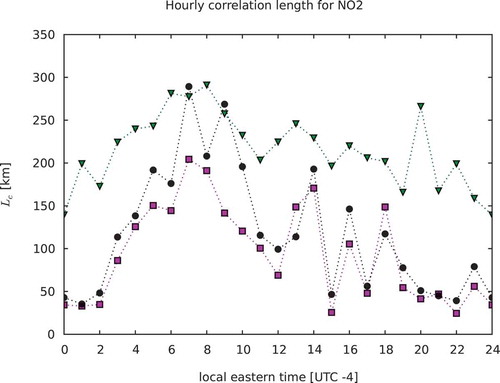
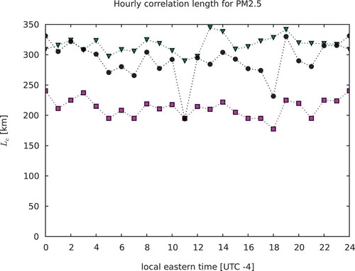
Figure 14. Time evolution of the correlation length for PM_2.5. Maximum likelihood estimates in pink, estimates in black, and global HL in green.