575
Views
1
CrossRef citations to date
0
Altmetric
Technical Papers

On dispersion above a forest—Measurements and methods

, &
Pages 768-785 | Received 25 Jan 2016, Accepted 24 Mar 2016, Published online: 22 Apr 2016

Figures & data

Table 1. The 61-m tower locations considered in this work.

Figure 1. The 61-m tower locations across the Savannah River National Laboratory reservation in South Carolina. In the present analysis, data from tower “D” are used most extensively. Tower “CS” is located in an area surrounded by buildings. Its data will not be used here.
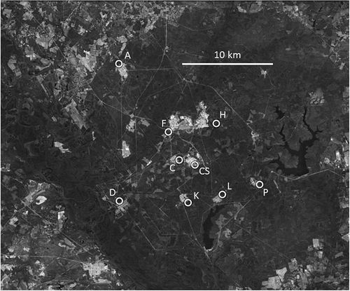
Figure 1. The 61-m tower locations across the Savannah River National Laboratory reservation in South Carolina. In the present analysis, data from tower “D” are used most extensively. Tower “CS” is located in an area surrounded by buildings. Its data will not be used here.

Table 2. Total number of 30-min averages within P-G categories, for different methods of categorization.

Figure 2. The variation of σθ and σϕ with stability category, determined using five different methods as identified: (1) using the 36-m σθ data, (2) 36-m σϕ, (3) 61-m σθ, (4) 61-m σϕ, and (5) SRDT (see text). The six bars for each case represent the results for P-G categories A, B, C, D, E, and F sequentially, starting from the left for each grouping. Data from tower “D” are used.
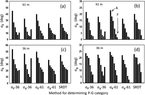
Figure 2. The variation of σθ and σϕ with stability category, determined using five different methods as identified: (1) using the 36-m σθ data, (2) 36-m σϕ, (3) 61-m σθ, (4) 61-m σϕ, and (5) SRDT (see text). The six bars for each case represent the results for P-G categories A, B, C, D, E, and F sequentially, starting from the left for each grouping. Data from tower “D” are used.

Figure 3. The coefficients of variation (CoV ≡ σχ/χ) corresponding to the values plotted in . Small values indicate a well-ordered statistical distribution. Values increase with an increasing contribution of randomness. Crosses identify cases in which the quantities plotted are sorted according to reported values of the same quantities, so that CoV values are necessarily small.
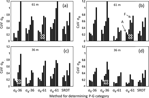
Figure 3. The coefficients of variation (CoV ≡ σχ/χ) corresponding to the values plotted in Figure 2. Small values indicate a well-ordered statistical distribution. Values increase with an increasing contribution of randomness. Crosses identify cases in which the quantities plotted are sorted according to reported values of the same quantities, so that CoV values are necessarily small.

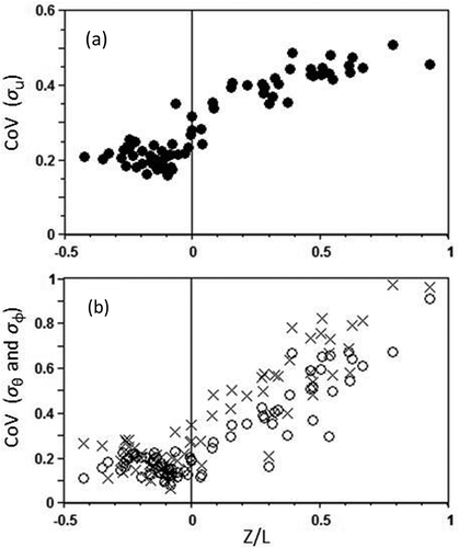
Figure 4. (a, b) Variation of σθ (a) and σϕ (b) with stability for tower “D” and (c, d) corresponding CoVs. Stability is quantified as (zd)/L, where z is the height above the ground, d is the zero-plane displacement, and L is the Obukhov length scale of turbulence. The heavier line represents data from 36 m, the lighter line, 61 m.
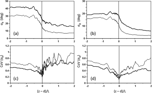
Figure 4. (a, b) Variation of σθ (a) and σϕ (b) with stability for tower “D” and (c, d) corresponding CoVs. Stability is quantified as (z − d)/L, where z is the height above the ground, d is the zero-plane displacement, and L is the Obukhov length scale of turbulence. The heavier line represents data from 36 m, the lighter line, 61 m.

Figure 5. As in , except that stability is now quantified as the Richardson number (Ri) derived using the 36-m and 61-m data.
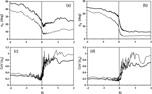
Figure 5. As in Figure 4, except that stability is now quantified as the Richardson number (Ri) derived using the 36-m and 61-m data.

Figure 6. As in and , but showing the dependence on time of day (as hours after sunrise).

Figure 6. As in Figures 4 and 5, but showing the dependence on time of day (as hours after sunrise).

Figure 7. (a, b) Dependence on wind speed of σθ (+) and σϕ (x) for the 61 m and 36 m heights, respectively. (c, d) Corresponding coefficients of variation.
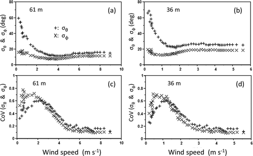
Figure 7. (a, b) Dependence on wind speed of σθ (+) and σϕ (x) for the 61 m and 36 m heights, respectively. (c, d) Corresponding coefficients of variation.

Figure 8. Velocity component statistics versus the relevant velocity scales. Each data point represents a 30-min sampling period. To simplify the presentation, every 25th data point after ordering according to wind speed is plotted. (a, c) σθ (+) and σϕ (o); (b, d) results using the same data set for σv and σw. The upper panels (a, b) are for the peak unstable hours (10:00 a.m. to 4:00 p.m.); the lower panels (c, d) for the peak hours of stable stratification (10:00 p.m. to 4:00 a.m.).
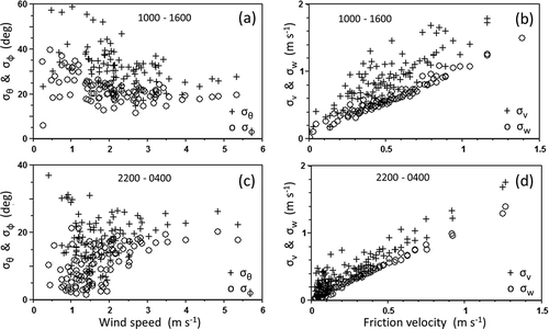
Figure 8. Velocity component statistics versus the relevant velocity scales. Each data point represents a 30-min sampling period. To simplify the presentation, every 25th data point after ordering according to wind speed is plotted. (a, c) σθ (+) and σϕ (o); (b, d) results using the same data set for σv and σw. The upper panels (a, b) are for the peak unstable hours (10:00 a.m. to 4:00 p.m.); the lower panels (c, d) for the peak hours of stable stratification (10:00 p.m. to 4:00 a.m.).

Figure 9. The variation of velocity component standard deviations with stability, represented by Ri. The solid lines link averages of 36-m data; the lighter lines, 61-m. (a, c) Transverse velocity (v) results; (b, d) vertical (w) component results. As in other figures, the lower panels (c, d) show the coefficients of variation corresponding to the upper panels. Note the difference between the 36-m data and the 61-m data in the case of σw, such difference is lacking in the case of σv.
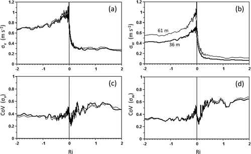
Figure 9. The variation of velocity component standard deviations with stability, represented by Ri. The solid lines link averages of 36-m data; the lighter lines, 61-m. (a, c) Transverse velocity (v) results; (b, d) vertical (w) component results. As in other figures, the lower panels (c, d) show the coefficients of variation corresponding to the upper panels. Note the difference between the 36-m data and the 61-m data in the case of σw, such difference is lacking in the case of σv.

Figure 10. The dependence on stability of two alternative quantifications of the standard deviations of (a) wind speed (u), (b) the lateral angular component (σθ), and (c) the vertical angular departure (σϕ). In each of the panels, circles indicate the average standard deviations in time (e.g., <σu>, plotted using the left hand axes) and the pluses the “meander” standard deviations determined from measurements of the corresponding quantities at the eight reporting stations (e.g., σ, referred to the axes on the right). Note that the vertical axes are the same in panel a, and also in panel b. However, in panel c, axis for σ() is scaled differently from that for <σϕ> because the average vertical velocity over each averaging period is close to zero and the standard deviation among these small values is itself necessarily small.
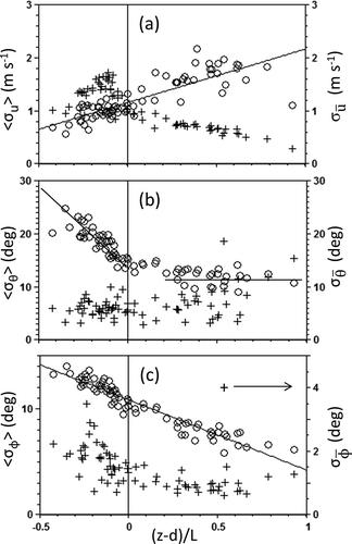
Figure 10. The dependence on stability of two alternative quantifications of the standard deviations of (a) wind speed (u), (b) the lateral angular component (σθ), and (c) the vertical angular departure (σϕ). In each of the panels, circles indicate the average standard deviations in time (e.g., <σu>, plotted using the left hand axes) and the pluses the “meander” standard deviations determined from measurements of the corresponding quantities at the eight reporting stations (e.g., σ, referred to the axes on the right). Note that the vertical axes are the same in panel a, and also in panel b. However, in panel c, axis for σ() is scaled differently from that for <σϕ> because the average vertical velocity over each averaging period is close to zero and the standard deviation among these small values is itself necessarily small.

Figure 11. The total effective standard deviations corresponding to the panels of , constructed by adding the time and space variances. Values of the amplification factor (A) that could be applied to the single-point estimates of the three different dispersion quantities are plotted as lines joining averages, as A − 1.
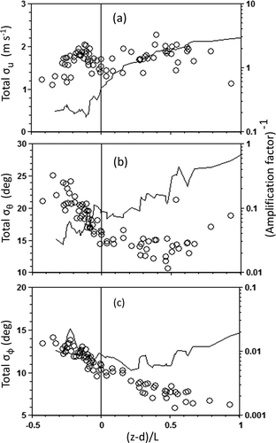
Figure 11. The total effective standard deviations corresponding to the panels of Figure 10, constructed by adding the time and space variances. Values of the amplification factor (A) that could be applied to the single-point estimates of the three different dispersion quantities are plotted as lines joining averages, as A − 1.
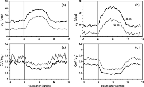
Figure 12. For the three quantities illustrated in and , the corresponding total CoVs derived by combining the variances in space and in time: for (a) σu; (b) σθ (crosses) and σϕ (circles).

Figure 12. For the three quantities illustrated in Figures 10 and 11, the corresponding total CoVs derived by combining the variances in space and in time: for (a) σu; (b) σθ (crosses) and σϕ (circles).

Reprints and Corporate Permissions

Please note: Selecting permissions does not provide access to the full text of the article, please see our help page How do I view content?

To request a reprint or corporate permissions for this article, please click on the relevant link below:

Academic Permissions

Please note: Selecting permissions does not provide access to the full text of the article, please see our help page How do I view content?

Obtain permissions instantly via Rightslink by clicking on the button below:

If you are unable to obtain permissions via Rightslink, please complete and submit this Permissions form. For more information, please visit our Permissions help page.