7,319
Views
63
CrossRef citations to date
0
Altmetric
Technical Papers

Comparison of real-time instruments and gravimetric method when measuring particulate matter in a residential building

, , , , , , & show all
Pages 1109-1120 | Received 04 Mar 2016, Accepted 08 Jun 2016, Published online: 22 Jun 2016

Figures & data

Table 1. Summary of PM2.5 measurements (μg/m3) from the different real-time and filter-based metrics.

Figure 1. Comparison of PM2.5 24 hr average concentrations between pDR-1500 direct reading and pDR-1500 filter-based measurements. The regression is presented by the following equation: y = β1(±SE)x + β0(±SE) where β1 and β0 are regression coefficients, and SE is the standard error of β values.
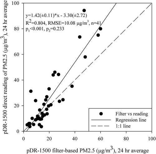
Figure 1. Comparison of PM2.5 24 hr average concentrations between pDR-1500 direct reading and pDR-1500 filter-based measurements. The regression is presented by the following equation: y = β1(±SE)x + β0(±SE) where β1 and β0 are regression coefficients, and SE is the standard error of β values.
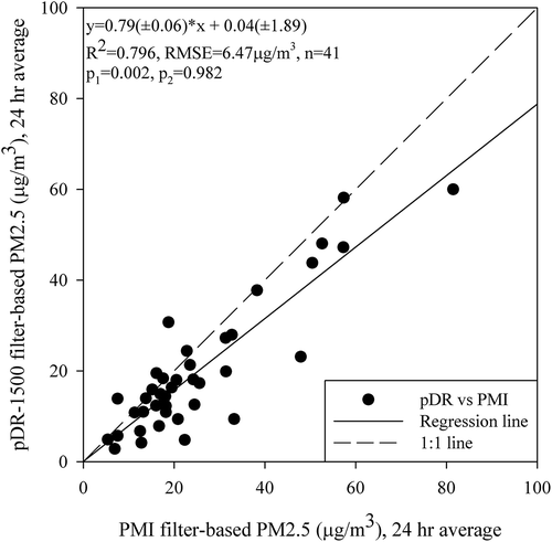
Figure 2. Comparison of PM2.5 24-hr average concentrations determined by PMI PM2.5 filter-based measurements and pDR-1500 filter-based measurements. The regression is presented by the following equation: y = β1(±SE)x + β0(±SE) where β1 and β0 are regression coefficients, and SE is the standard error of β values.
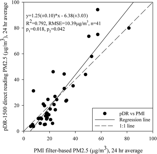
Figure 2. Comparison of PM2.5 24-hr average concentrations determined by PMI PM2.5 filter-based measurements and pDR-1500 filter-based measurements. The regression is presented by the following equation: y = β1(±SE)x + β0(±SE) where β1 and β0 are regression coefficients, and SE is the standard error of β values.
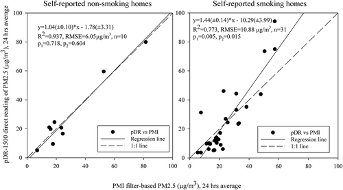
Figure 3. Comparison of PM2.5 24-hr average concentrations determined by PMI PM2.5 filter-based measurements and pDR-1500 direct reading measurements. The regression is presented by the following equation: y = β1(±SE)x + β0(±SE) where β1 and β0 are regression coefficients, and SE is the standard error of β values.
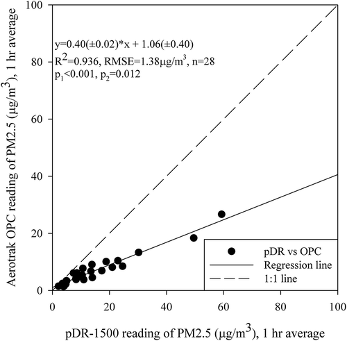
Figure 3. Comparison of PM2.5 24-hr average concentrations determined by PMI PM2.5 filter-based measurements and pDR-1500 direct reading measurements. The regression is presented by the following equation: y = β1(±SE)x + β0(±SE) where β1 and β0 are regression coefficients, and SE is the standard error of β values.
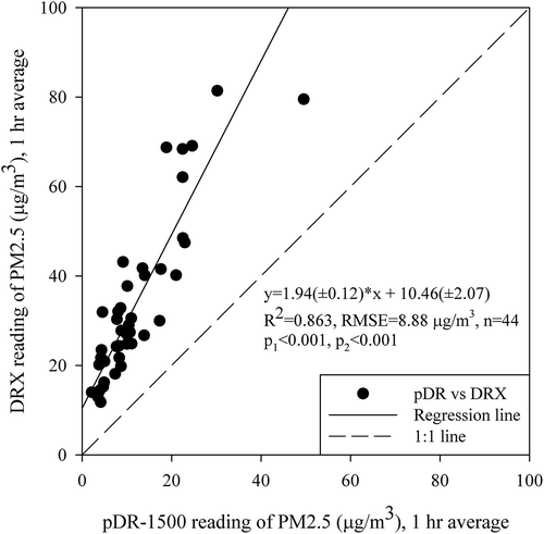
Figure 4. Comparison of PM2.5 24 hr average concentrations determined by PMI PM2.5 filter-based measurements and pDR-1500 direct reading measurements, with data stratified according to the self-reported smoking status in investigated apartments. The regression is presented by the following equation: y = β1(±SE)x + β0(±SE) where β1 and β0 are regression coefficients, and SE is the standard error of β values.

Figure 4. Comparison of PM2.5 24 hr average concentrations determined by PMI PM2.5 filter-based measurements and pDR-1500 direct reading measurements, with data stratified according to the self-reported smoking status in investigated apartments. The regression is presented by the following equation: y = β1(±SE)x + β0(±SE) where β1 and β0 are regression coefficients, and SE is the standard error of β values.

Figure 5. Comparison of PM2.5 1-hr average concentrations determined by pDR-1500 direct reading measurements and Aerotrak OPC estimate assuming particles are spherical and have a density of 1.68 g/cm3. The regression is presented by the following equation: y = β1(±SE)x + β0(±SE) where β1 and β0 are regression coefficients, and SE is the standard error of β values.

Figure 5. Comparison of PM2.5 1-hr average concentrations determined by pDR-1500 direct reading measurements and Aerotrak OPC estimate assuming particles are spherical and have a density of 1.68 g/cm3. The regression is presented by the following equation: y = β1(±SE)x + β0(±SE) where β1 and β0 are regression coefficients, and SE is the standard error of β values.

Figure 6. Comparison of PM2.5 1-hr average concentrations determined by pDR-1500 and DustTrak DRX direct reading measurements. The regression is presented by the following equation: y = β1(±SE)x + β0(±SE) where β1 and β0 are regression coefficients, and SE is the standard error of β values.

Figure 6. Comparison of PM2.5 1-hr average concentrations determined by pDR-1500 and DustTrak DRX direct reading measurements. The regression is presented by the following equation: y = β1(±SE)x + β0(±SE) where β1 and β0 are regression coefficients, and SE is the standard error of β values.

Reprints and Corporate Permissions

Please note: Selecting permissions does not provide access to the full text of the article, please see our help page How do I view content?

To request a reprint or corporate permissions for this article, please click on the relevant link below:

Academic Permissions

Please note: Selecting permissions does not provide access to the full text of the article, please see our help page How do I view content?

Obtain permissions instantly via Rightslink by clicking on the button below:

If you are unable to obtain permissions via Rightslink, please complete and submit this Permissions form. For more information, please visit our Permissions help page.